Correlating Like a Data Master

Purpose of this chapter

Assess relationships within a novel data set using publication quality tables and plots

---

Take-aways

1. Describe and visualize correlations between numerical variables
2. Visualize correlations of all numerical variables within groups
3. Describe and visualize relationships based on target variables

---

Required setup

We first need to prepare our environment with the necessary packages.

if (!require(pacman))
  install.packages("pacman")

pacman::p_load(colorblindr,
       dlookr,
       formattable,
       GGally,
       ggdist,
       ggpubr,
       ggridges,
       here,
       tidyverse)

# Set global ggplot() theme
# Theme pub_clean() from the ggpubr package with base text size = 16
theme_set(theme_pubclean(base_size = 12)) 
# All axes titles to their respective far right sides
theme_update(axis.title = element_text(hjust = 1))
# Remove axes ticks
theme_update(axis.ticks = element_blank()) 
# Remove legend key
theme_update(legend.key = element_blank())

---

Load the Examine a Data Set

We will be using open source data from UArizona researchers that investigates the effects of climate change on canopy trees. (Meredith, Ladd, and Werner 2021)

# Let's load the canopy tree data set
dataset <- read.csv(here("EDA_In_R_Book", "data", "Data_Fig2_Repo.csv"))

# What does the data look like?
dataset |>
  head() |>
  formattable()

Date	Group	Sap_Flow	TWaterFlux	pLWP	mLWP
10/4/19	Drought-sens-canopy	184.040975	82.243292	-0.2633781	-0.6797690
10/4/19	Drought-sens-under	2.475989	1.258050	-0.2996688	-0.7613264
10/4/19	Drought-tol-canopy	10.598949	4.405479	-0.4375563	-0.7225572
10/4/19	Drought-tol-under	4.399854	2.055276	-0.2052237	-0.7028581
10/5/19	Drought-sens-canopy	182.905444	95.865255	-0.2769280	-0.7082610
10/5/19	Drought-sens-under	2.459209	1.225792	-0.3205980	-0.7928576

---

Describe and Visualize Correlations

Correlations are a statistical relationship between two numerical variables, may or may not be causal. Exploring correlations in your data allows you determine data independence, a major assumption of parametric statistics, which means your variables are both randomly collected.

If you’re interested in some underlying statistics…

Note that the dlookr default correlation is the Pearson’s \(r\) coefficient, but you can specify any method you would like: correlate(dataset, method = ""), where the method can be "pearson" for Pearson’s \(r\), "spearman" for Spearman’s \(\rho\), or "kendall" for Kendall’s \(\tau\). The main differences are that Pearson’s \(r\) assumes a normal distribution for ALL numerical variables, whereas Spearman’s \(\rho\) and Kendall’s \(\tau\) do not, but Spearman’s \(\rho\) requires \(N > 10\), and Kendall’s \(\tau\) does not. Notably, Kendall’s \(\tau\) performs as well as Spearman’s \(\rho\) when \(N > 10\), so its best to just use Kendall’s \(\tau\) when data are not normally distributed.

# Table of correlations between numerical variables (we are sticking to the default Pearson's r coefficient)
correlate(dataset) |>
  formattable()

var1	var2	coef_corr
TWaterFlux	Sap_Flow	0.9881370
pLWP	Sap_Flow	0.1202809
mLWP	Sap_Flow	-0.2011949
Sap_Flow	TWaterFlux	0.9881370
pLWP	TWaterFlux	0.1256446
mLWP	TWaterFlux	-0.1893302
Sap_Flow	pLWP	0.1202809
TWaterFlux	pLWP	0.1256446
mLWP	pLWP	0.6776509
Sap_Flow	mLWP	-0.2011949
TWaterFlux	mLWP	-0.1893302
pLWP	mLWP	0.6776509

# Correlation matrix of numerical variables
dataset |>
plot_correlate()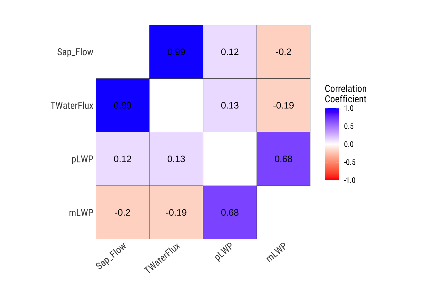

---

Visualize Correlations within Groups

If we have groups that we will compare later on, it is a good idea to see how each numerical variable correlates within these groups.

dataset |>
  group_by(Group) |>
  plot_correlate()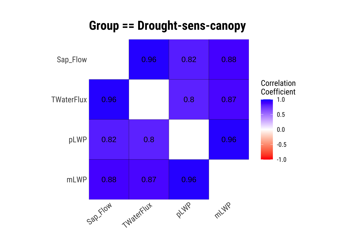

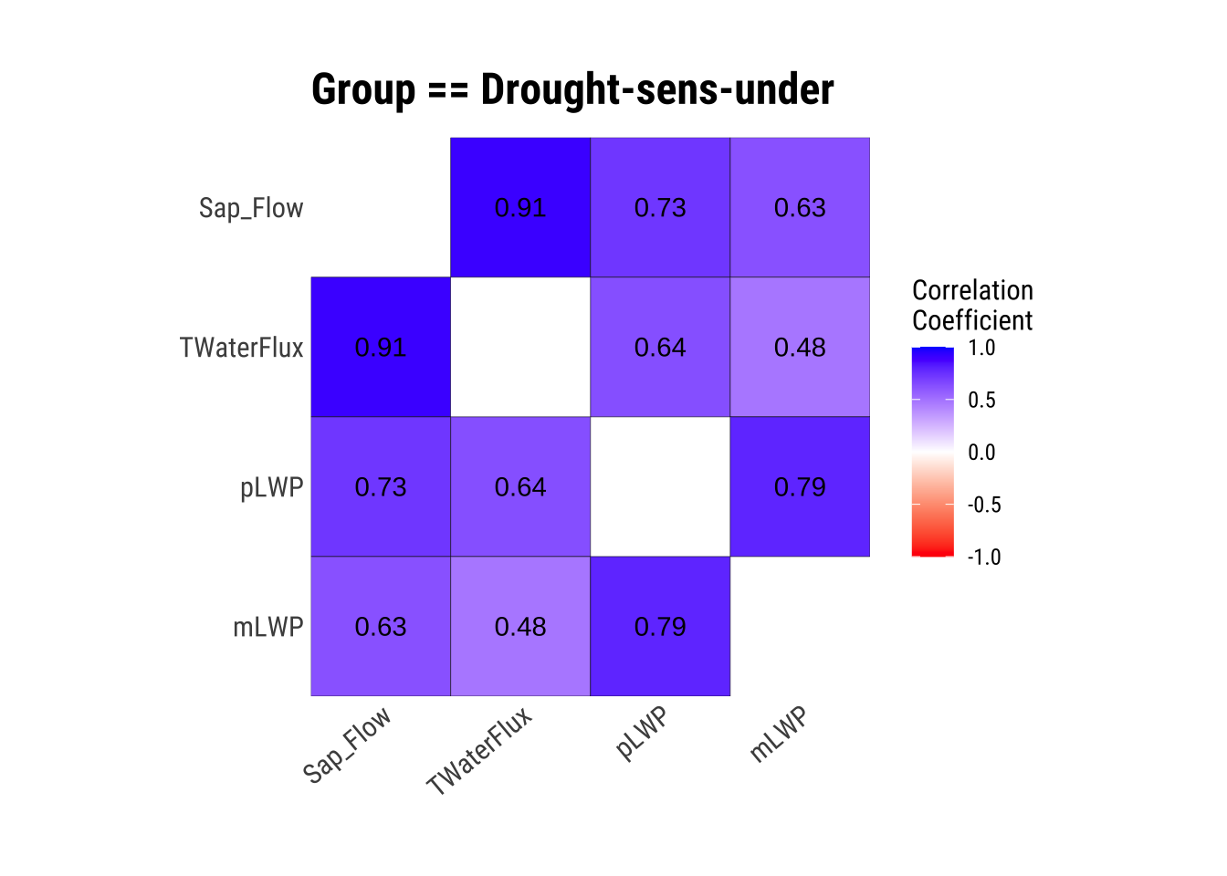
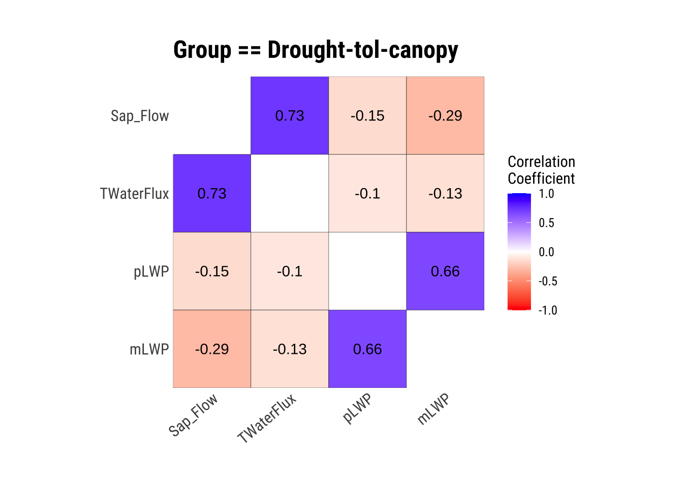
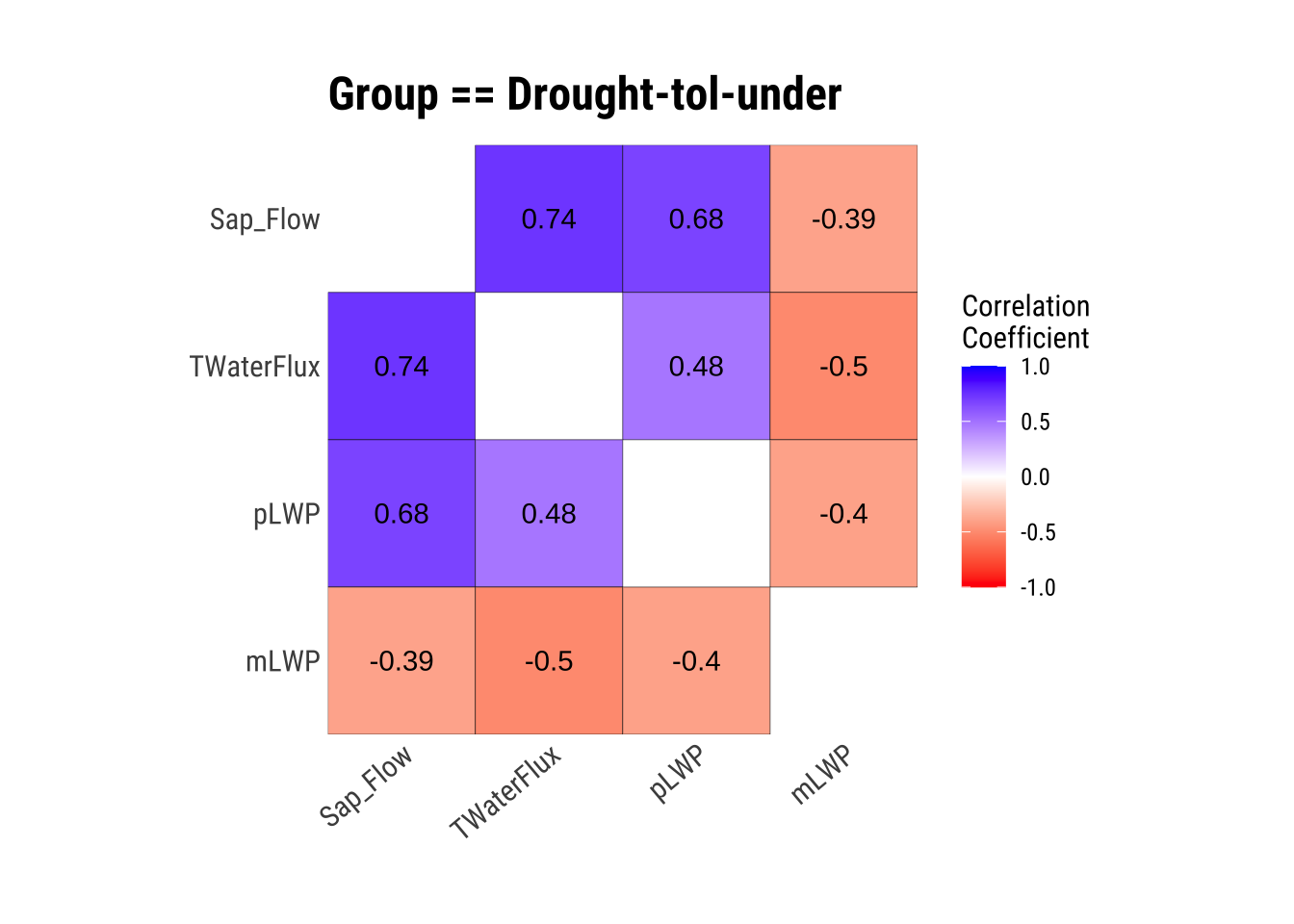
This is great, we have our correlations within groups! However, the correlation matrices aren’t always the most intuitive, so let’s plot!

We will be using the ggpairs() function within the GGally package. Specifically, we are looking at the correlations between predawn leaf water potential pLWP and midday leaf water potential mLWP. Leaf water potential is a key indicator for how stressed plants are in droughts.

dataset |> 
  dplyr::select(Group, pLWP, mLWP) |>
  ggpairs(aes(color = Group, alpha = 0.5)) +
  theme(strip.background = element_blank()) + # I don't like facet strip backgrounds...
  scale_fill_OkabeIto() +
  scale_color_OkabeIto()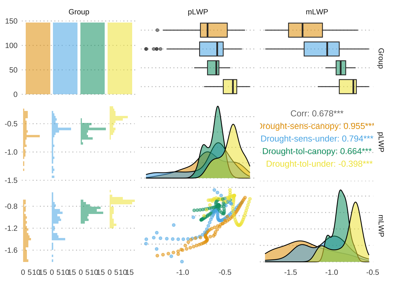

---

Describe and Visualize Relationships Based on Target Variables

Target Variables

Target variables are essentially numerical or categorical variables that you want to relate others to in a data frame. dlookr does this through the target_by() function, which is similar to group_by() in dplyr. The relate() function then briefly analyzes the relationship between the target variable and the variables of interest.

The relationships below will have the formula relationship target ~ predictor.

---

Numerical Target Variables: Numerical Variable of Interest

Formula: Sap_Flow (numerical response) ~ pLWP (numerical predictor)

# First, we need to remove NAs, they cause an error
dataset.noNA <- dataset |> 
  drop_na()

# The numerical predictor variable that we want
num <- target_by(dataset.noNA, Sap_Flow)

# Relating the variable of interest to the numerical target variable
num_num <- relate(num, pLWP)

# Summary of the regression analysis - the same as the summary from lm(Formula)
summary(num_num)

Call:
lm(formula = formula_str, data = data)

Residuals:
    Min      1Q  Median      3Q     Max 
-32.719 -26.647 -20.924  -0.811 148.353 

Coefficients:
            Estimate Std. Error t value Pr(>|t|)    
(Intercept)   42.167      7.971   5.290 2.51e-07 ***
pLWP          24.600     12.266   2.006   0.0459 *  
---
Signif. codes:  0 '***' 0.001 '**' 0.01 '*' 0.05 '.' 0.1 ' ' 1

Residual standard error: 46.2 on 274 degrees of freedom
Multiple R-squared:  0.01447,   Adjusted R-squared:  0.01087 
F-statistic: 4.022 on 1 and 274 DF,  p-value: 0.04589

# Plotting the linear relationship
plot(num_num)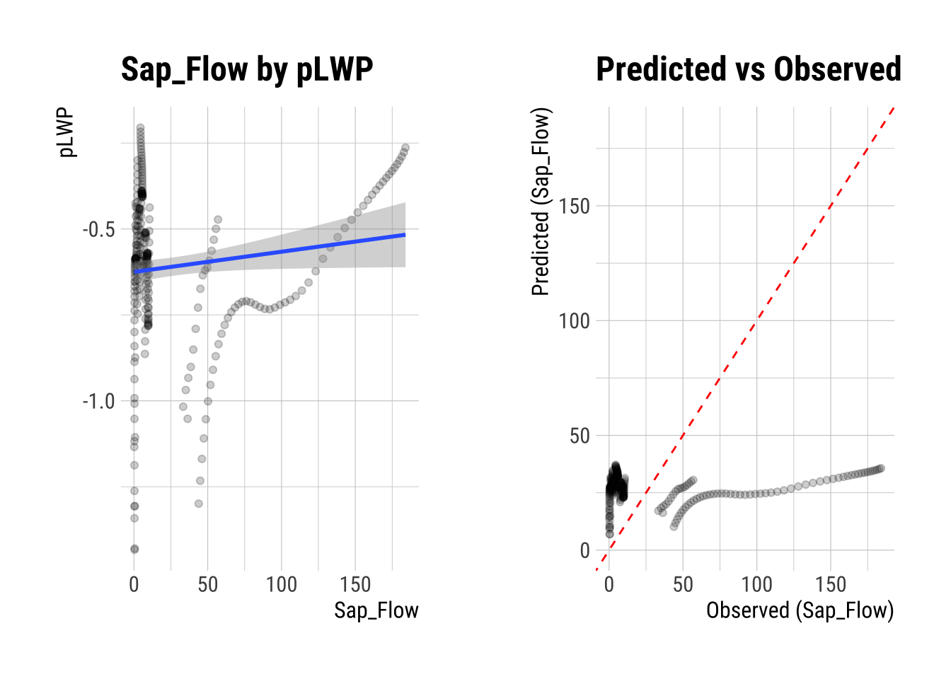

---

Numerical Target Variables: Categorical Variable of Interest

Formula: pLWP (numerical response) ~ Group (categorical predictor)

# The categorical predictor variable that we want
num <- target_by(dataset, pLWP) 

# We need to change Group to a factor
num$Group <- as.factor(num$Group)

# Relating the variable of interest to the numerical target variable
num_cat <- relate(num, Group)

# Summary of the ANOVA analysis - the same as the summary from anova(lm(Formula))
summary(num_cat)

Call:
lm(formula = formula(formula_str), data = data)

Residuals:
     Min       1Q   Median       3Q      Max 
-0.73720 -0.09700  0.03598  0.11314  0.40655 

Coefficients:
                        Estimate Std. Error t value Pr(>|t|)    
(Intercept)             -0.66993    0.02466 -27.166  < 2e-16 ***
GroupDrought-sens-under -0.02621    0.03488  -0.751    0.453    
GroupDrought-tol-canopy  0.04002    0.03488   1.148    0.252    
GroupDrought-tol-under   0.22969    0.03488   6.586 2.33e-10 ***
---
Signif. codes:  0 '***' 0.001 '**' 0.01 '*' 0.05 '.' 0.1 ' ' 1

Residual standard error: 0.2048 on 272 degrees of freedom
  (312 observations deleted due to missingness)
Multiple R-squared:  0.1956,    Adjusted R-squared:  0.1867 
F-statistic: 22.05 on 3 and 272 DF,  p-value: 8.267e-13

plot(num_cat) + 
  theme(axis.text.x = element_blank())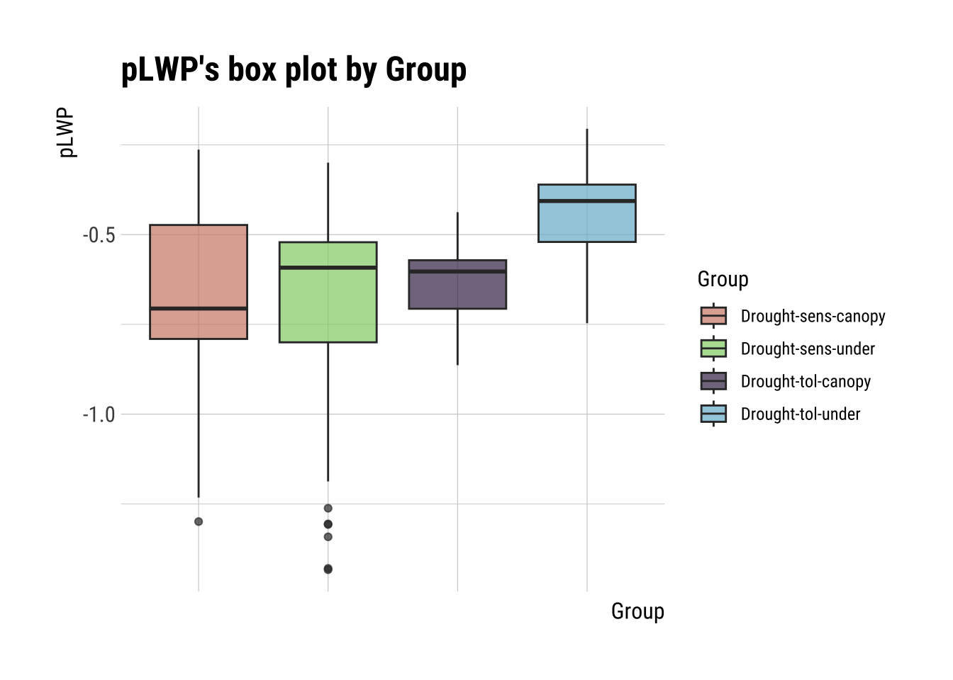

---

Categorical Target Variables: Numerical Variable of Interest

Note that this produces descriptive statistics, unlike the other relationships we are looking at.

Formula: Group (categorical) ~ pLWP (numerical)

# The categorical predictor variable that we want
categ <- target_by(dataset, Group)

# Relating the variable of interest to the numerical target variable
cat_num <- relate(categ, pLWP)

# Summary of descriptive statistics
summary(cat_num)

 described_variables    Group                 n               na       
 Length:5            Length:5           Min.   : 69.0   Min.   : 78.0  
 Class :character    Class :character   1st Qu.: 69.0   1st Qu.: 78.0  
 Mode  :character    Mode  :character   Median : 69.0   Median : 78.0  
                                        Mean   :110.4   Mean   :124.8  
                                        3rd Qu.: 69.0   3rd Qu.: 78.0  
                                        Max.   :276.0   Max.   :312.0  
      mean               sd             se_mean             IQR        
 Min.   :-0.6961   Min.   :0.09557   Min.   :0.01151   Min.   :0.1351  
 1st Qu.:-0.6699   1st Qu.:0.13188   1st Qu.:0.01367   1st Qu.:0.1597  
 Median :-0.6299   Median :0.22715   Median :0.01588   Median :0.2640  
 Mean   :-0.6091   Mean   :0.19699   Mean   :0.02098   Mean   :0.2310  
 3rd Qu.:-0.6091   3rd Qu.:0.24639   3rd Qu.:0.02966   3rd Qu.:0.2788  
 Max.   :-0.4402   Max.   :0.28394   Max.   :0.03418   Max.   :0.3173  
    skewness          kurtosis            p00               p01         
 Min.   :-1.1510   Min.   :-0.5921   Min.   :-1.4333   Min.   :-1.4307  
 1st Qu.:-1.1047   1st Qu.:-0.4320   1st Qu.:-1.4333   1st Qu.:-1.3160  
 Median :-0.4644   Median :-0.2744   Median :-1.2993   Median :-1.2538  
 Mean   :-0.7009   Mean   : 0.1897   Mean   :-1.1553   Mean   :-1.1133  
 3rd Qu.:-0.4333   3rd Qu.: 0.4796   3rd Qu.:-0.8637   3rd Qu.:-0.8388  
 Max.   :-0.3510   Max.   : 1.7675   Max.   :-0.7467   Max.   :-0.7272  
      p05               p10               p20               p25         
 Min.   :-1.3067   Min.   :-1.1449   Min.   :-0.9067   Min.   :-0.8000  
 1st Qu.:-1.0870   1st Qu.:-1.0047   1st Qu.:-0.8587   1st Qu.:-0.7906  
 Median :-1.0666   Median :-0.8802   Median :-0.7339   Median :-0.7140  
 Mean   :-0.9838   Mean   :-0.8878   Mean   :-0.7583   Mean   :-0.7063  
 3rd Qu.:-0.7816   3rd Qu.:-0.7724   3rd Qu.:-0.7304   3rd Qu.:-0.7065  
 Max.   :-0.6772   Max.   :-0.6366   Max.   :-0.5619   Max.   :-0.5205  
      p30               p40               p50               p60         
 Min.   :-0.7386   Min.   :-0.7204   Min.   :-0.7059   Min.   :-0.6206  
 1st Qu.:-0.7076   1st Qu.:-0.6299   1st Qu.:-0.6028   1st Qu.:-0.5861  
 Median :-0.6801   Median :-0.6292   Median :-0.5921   Median :-0.5855  
 Mean   :-0.6590   Mean   :-0.6079   Mean   :-0.5787   Mean   :-0.5487  
 3rd Qu.:-0.6790   3rd Qu.:-0.6171   3rd Qu.:-0.5862   3rd Qu.:-0.5536  
 Max.   :-0.4896   Max.   :-0.4427   Max.   :-0.4064   Max.   :-0.3978  
      p70               p75               p80               p90         
 Min.   :-0.5758   Min.   :-0.5714   Min.   :-0.5653   Min.   :-0.5150  
 1st Qu.:-0.5504   1st Qu.:-0.5212   1st Qu.:-0.4907   1st Qu.:-0.4243  
 Median :-0.5269   Median :-0.4733   Median :-0.4259   Median :-0.3519  
 Mean   :-0.5068   Mean   :-0.4753   Mean   :-0.4446   Mean   :-0.3812  
 3rd Qu.:-0.4925   3rd Qu.:-0.4500   3rd Qu.:-0.4088   3rd Qu.:-0.3394  
 Max.   :-0.3883   Max.   :-0.3608   Max.   :-0.3325   Max.   :-0.2756  
      p95               p99               p100        
 Min.   :-0.5100   Min.   :-0.4609   Min.   :-0.4376  
 1st Qu.:-0.3700   1st Qu.:-0.3139   1st Qu.:-0.2997  
 Median :-0.3049   Median :-0.2726   Median :-0.2634  
 Mean   :-0.3457   Mean   :-0.2994   Mean   :-0.2822  
 3rd Qu.:-0.3004   3rd Qu.:-0.2363   3rd Qu.:-0.2052  
 Max.   :-0.2430   Max.   :-0.2133   Max.   :-0.2052  

plot(cat_num)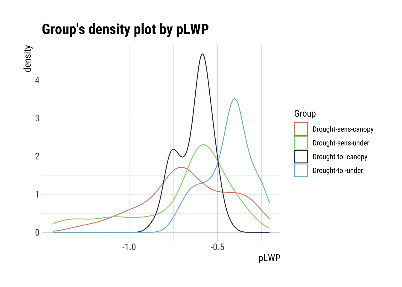 

---

Categorical Target Variables: Categorical Variable of Interest

Notably, there is only one categorical variable… Let’s make another:

If \(mLWP > mean(mLWP) + sd(mLWP)\) then “Yes”, else “No”.

# Create new categorical column
cat_dataset <- dataset |>
  select(pLWP, Group) |>
  drop_na() |>
  mutate(HighLWP = ifelse(
    pLWP > (mean(pLWP + sd(pLWP))), 
                          "Yes", 
                          "No"))

# New dataset 
cat_dataset |>
  head() |>
  formattable()

pLWP	Group	HighLWP
-0.2633781	Drought-sens-canopy	Yes
-0.2996688	Drought-sens-under	Yes
-0.4375563	Drought-tol-canopy	No
-0.2052237	Drought-tol-under	Yes
-0.2769280	Drought-sens-canopy	Yes
-0.3205980	Drought-sens-under	Yes

Now we have two categories!

Formula = HighLWP (categorical) ~ Group (categorical response)

# The categorical predictor variable that we want
categ <- target_by(cat_dataset, HighLWP)

# Relating the variable of interest to the categorical target variable
cat_cat <- relate(categ, Group)

# Summary of the Chi-square test for Independence
summary(cat_cat)

Call: xtabs(formula = formula_str, data = data, addNA = TRUE)
Number of cases in table: 276 
Number of factors: 2 
Test for independence of all factors:
    Chisq = 30.201, df = 3, p-value = 1.252e-06

plot(cat_cat)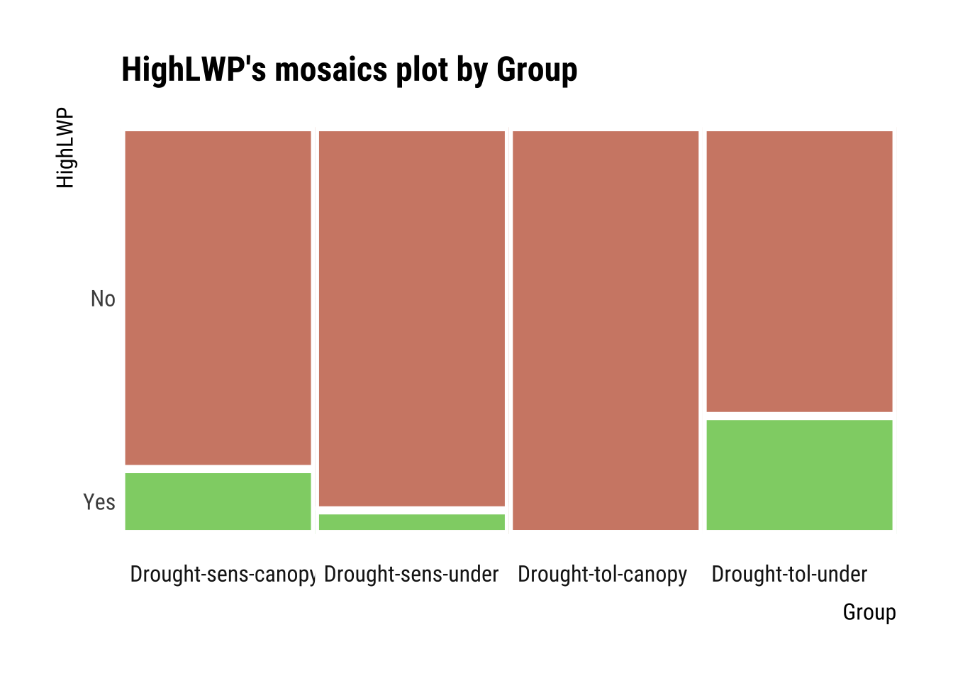

---

Meredith, Laura, S. Nemiah Ladd, and Christiane Werner. 2021. “Data for "Ecosystem Fluxes During Drought and Recovery in an Experimental Forest".” University of Arizona Research Data Repository. https://doi.org/10.25422/AZU.DATA.14632593.V1.