Correlating Like a Data Master

Purpose of this chapter

Assess relationships within a novel data set

---

Take-aways

1. Describe and visualize correlations between numerical variables
2. Visualize correlations of all numerical variables within groups
3. Describe and visualize relationships based on target variables

---

Required setup

We first need to prepare our environment with the necessary libraries and set a global theme for publishable plots in seaborn.

# Import all required libraries
# Data analysis and manipulation
import pandas as pd
# Working with arrays
import numpy as np
# Statistical visualization
import seaborn as sns
# Matlab plotting for Python
import matplotlib.pyplot as plt
import matplotlib.patches as mpatches
# Data analysis
import statistics as stat
import scipy.stats as stats
# Two-sample Chi-Square test
from scipy.stats import chi2_contingency
# Predictive data analysis: process data 
from sklearn import preprocessing as pproc
# Predictive data analysis: linear models
from sklearn.model_selection import cross_val_predict
# Predictive data analysis: linear models
from sklearn.linear_model import LinearRegression
# Visualizing missing values
import missingno as msno
# Statistical modeling
import statsmodels.api as sm
# Statistical modeling: ANOVA
from statsmodels.formula.api import ols
# Mosaic plot
from statsmodels.graphics.mosaicplot import mosaic
from itertools import product

# Increase font and figure size of all seaborn plot elements
sns.set(font_scale = 1.5, rc = {'figure.figsize':(8, 8)})

# Change theme to "white"
sns.set_style("white")

---

Load the Examine a Data Set

We will be using open source data from UArizona researchers that investigates the effects of climate change on canopy trees. (Meredith, Ladd, and Werner 2021)

# Read csv 
data = pd.read_csv("data/Data_Fig2_Repo.csv")

# Convert 'Date' column to datetime
data['Date'] = pd.to_datetime(data['Date'])

# What does the data look like
data.head()

        Date                Group    Sap_Flow  TWaterFlux      pLWP      mLWP
0 2019-10-04  Drought-sens-canopy  184.040975   82.243292 -0.263378 -0.679769
1 2019-10-04   Drought-sens-under    2.475989    1.258050 -0.299669 -0.761326
2 2019-10-04   Drought-tol-canopy   10.598949    4.405479 -0.437556 -0.722557
3 2019-10-04    Drought-tol-under    4.399854    2.055276 -0.205224 -0.702858
4 2019-10-05  Drought-sens-canopy  182.905444   95.865255 -0.276928 -0.708261

---

Describe and Visualize Correlations

Correlations are a statistical relationship between two numerical variables, may or may not be causal. Exploring correlations in your data allows you determine data independence, a major assumption of parametric statistics, which means your variables are both randomly collected.

If you’re interested in some underlying statistics…

Note that the we will use the Pearson’s \(r\) coefficient in corr() function from the pandas library, but you can specify any method you would like: corr(method = ""), where the method can be "pearson" for Pearson’s \(r\), "spearman" for Spearman’s \(\rho\), or "kendall" for Kendall’s \(\tau\). The main differences are that Pearson’s \(r\) assumes a normal distribution for ALL numerical variables, whereas Spearman’s \(\rho\) and Kendall’s \(\tau\) do not, but Spearman’s \(\rho\) requires \(N > 10\), and Kendall’s \(\tau\) does not. Notably, Kendall’s \(\tau\) performs as well as Spearman’s \(\rho\) when \(N > 10\), so its best to just use Kendall’s \(\tau\) when data are not normally distributed.

# subset dataframe to include only numeric columns
numData = data.select_dtypes(include='number')

# Table of correlations between numerical variables (we are sticking to the default Pearson's r coefficient)
numData.corr()

            Sap_Flow  TWaterFlux      pLWP      mLWP
Sap_Flow    1.000000    0.988137  0.120281 -0.201195
TWaterFlux  0.988137    1.000000  0.125645 -0.189330
pLWP        0.120281    0.125645  1.000000  0.677651
mLWP       -0.201195   -0.189330  0.677651  1.000000

# Heatmap correlation matrix of numerical variables
# Correlation matrix
corr = numData.corr()

# Generate a mask for the upper triangle
mask = np.triu(np.ones_like(corr, dtype = bool))

# Generate a custom diverging colormap
cmap = sns.diverging_palette(230, 20, as_cmap = True)

# Heatmap of the correlation matrix
sns.heatmap(corr, cmap = cmap, mask = mask, vmax = 0.3, center = 0,
            square = True, linewidths = 0.5, cbar_kws = {"shrink": .5})
            
# Tight margins for plot
plt.tight_layout()

# Show plot
plt.show()

---

Visualize Correlations within Groups

If we have groups that we will compare later on, it is a good idea to see how each numerical variable correlates within these groups.

# Increase font and figure size of all seaborn plot elements
sns.set(font_scale = 1.5, rc = {'figure.figsize':(10, 10)})

# Change theme to "white"
sns.set_style("white")

# Heatmap correlation matrix of numerical variables
# Correlation matrix
corr = data.groupby('Group').corr()

# Generate a mask for the upper triangle
mask = np.triu(np.ones_like(corr, dtype = bool))

# Generate a custom diverging colormap
cmap = sns.diverging_palette(230, 20, as_cmap = True)

# Heatmap of the correlation matrix
ax = sns.heatmap(corr, cmap = cmap, mask = mask, vmax = 0.3, center = 0,
            square = True, linewidths = 0.5, cbar_kws = {"shrink": .5})
            
# Change y-axis label
ax.set(ylabel = 'Group')

# Tight margins for plot
plt.tight_layout()

# Show plot
plt.show()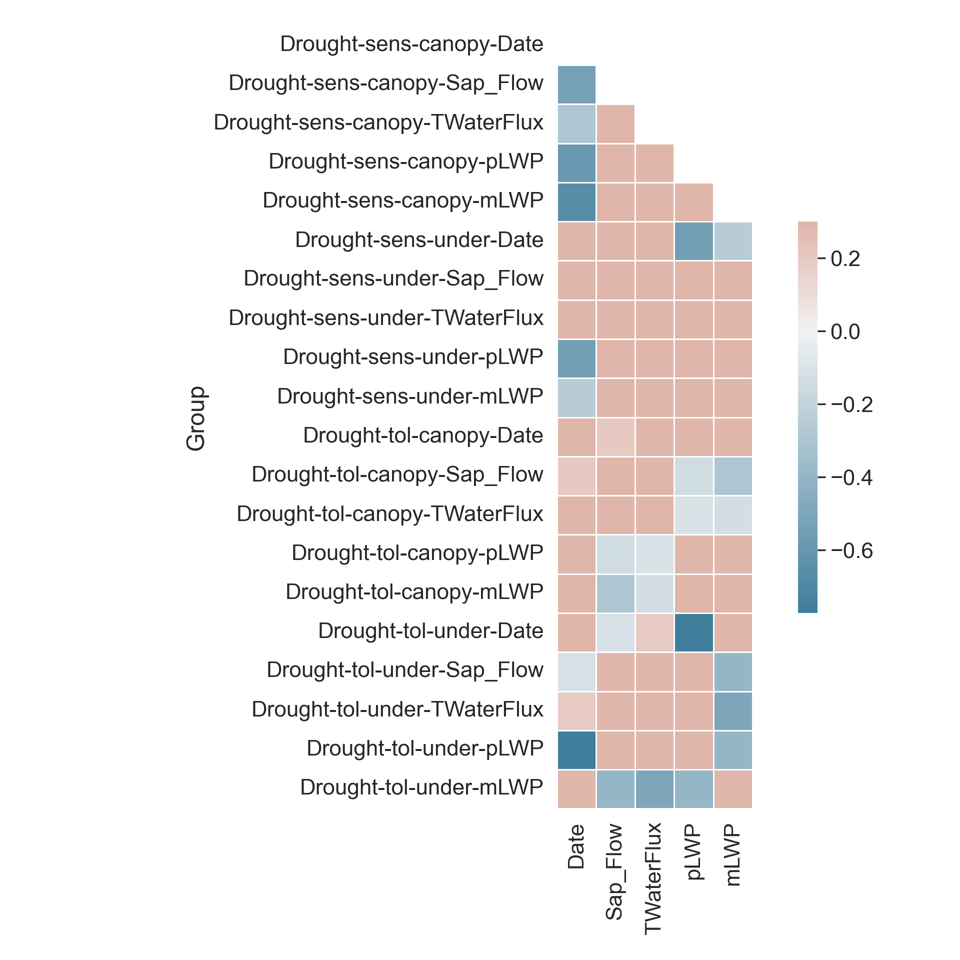

This is great, we have our correlations within groups! However, the correlation matrices aren’t always the most intuitive, so let’s plot!

Specifically, we are looking at the correlations between predawn leaf water potential pLWP and midday leaf water potential mLWP. Leaf water potential is a key indicator for how stressed plants are in droughts.

dataplot = data[["Group", "pLWP", "mLWP"]]

# Increase font and figure size of all seaborn plot elements
sns.set(font_scale = 2.5, rc = {'figure.figsize':(10, 10)})

# Change seaborn plot theme to white
sns.set_style("white")

# Empty subplot grid for pairwise relationships
g = sns.PairGrid(dataplot, hue = "Group", height = 5)

# Add scatterplots to the upper portion of the grid
g1 = g.map_upper(sns.scatterplot, alpha = 0.5, s = 100)

# Add a kernal density plot to the diagonal of the grid
g2 = g1.map_diag(sns.kdeplot, fill = True, linewidth = 3)

# Add a kernal density plot to the lower portion of the grid
g3 = g2.map_lower(sns.kdeplot, levels = 5, alpha = 0.75)

# Remove legend title
g4 = g3.add_legend(title = "", adjust_subtitles = True)

# Show plot
plt.show()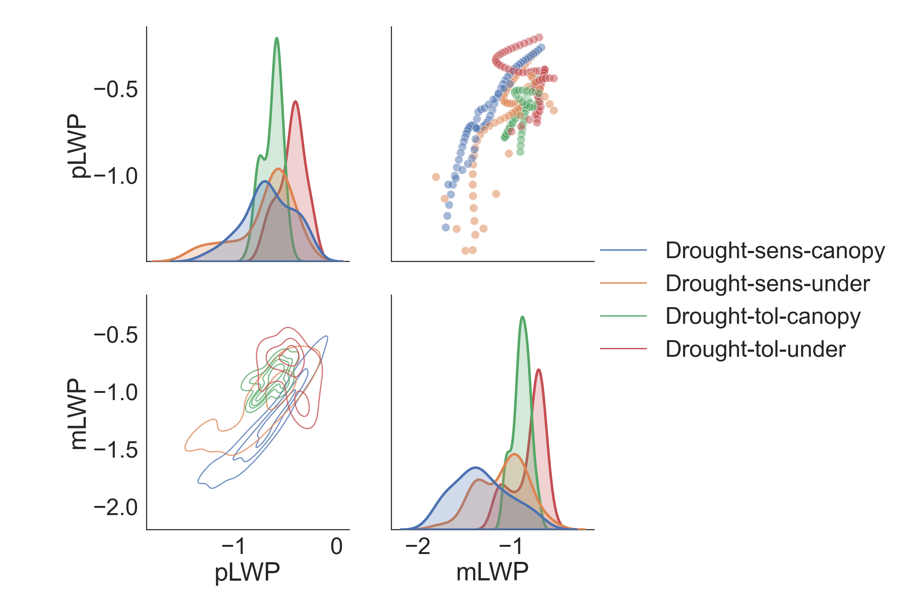

---

Describe and Visualize Relationships Based on Target Variables

Target Variables

Target variables are essentially numerical or categorical variables that you want to relate others to in a data frame.

The relationships below will have the formula relationship target ~ predictor.

---

Numerical Target Variables: Numerical Variable of Interest

Formula: pLWP (numerical) ~ mLWP (numerical)

# The numerical predictor variable 
X = data[["mLWP"]]

# The numerical target variable
Y = data[["pLWP"]]

# Define the linear model, drop NAs
model = sm.OLS(Y, X, missing = 'drop')

# Fit the model
model_result = model.fit()

# Summary of the linear model
model_result.summary()

OLS Regression Results

Dep. Variable:	pLWP	R-squared (uncentered):	0.934
Model:	OLS	Adj. R-squared (uncentered):	0.934
Method:	Least Squares	F-statistic:	3882.
Date:	Fri, 15 Sep 2023	Prob (F-statistic):	3.29e-164
Time:	00:40:16	Log-Likelihood:	102.11
No. Observations:	276	AIC:	-202.2
Df Residuals:	275	BIC:	-198.6
Df Model:	1
Covariance Type:	nonrobust

	coef	std err	t	P>|t|	[0.025	0.975]
mLWP	0.5995	0.010	62.309	0.000	0.581	0.618

Omnibus:	6.825	Durbin-Watson:	1.348
Prob(Omnibus):	0.033	Jarque-Bera (JB):	8.247
Skew:	-0.219	Prob(JB):	0.0162
Kurtosis:	3.725	Cond. No.	1.00

Notes:
[1] R² is computed without centering (uncentered) since the model does not contain a constant.
[2] Standard Errors assume that the covariance matrix of the errors is correctly specified.

# Plotting the linear relationship

# Increase font and figure size of all seaborn plot elements
sns.set(font_scale = 1.25, rc = {'figure.figsize':(8, 8)})

# Change seaborn plot theme to white
sns.set_style("white")

# Subplots
fig, (ax1, ax2) = plt.subplots(ncols = 2, nrows = 1)

# Regression plot between mLWP and pLWP
sns.regplot(data = data, x = "mLWP", y = "pLWP", ax = ax1)

# Set regression plot title
ax1.set_title("Linear regression")

# Regression plot between mLWP and pLWP
sns.residplot(data = data, x = "mLWP",
              y = "pLWP", ax = ax2)
              
# Set residual plot title
ax2.set_title("Residuals")

# Tight margins
plt.tight_layout()

# Show plot
plt.show()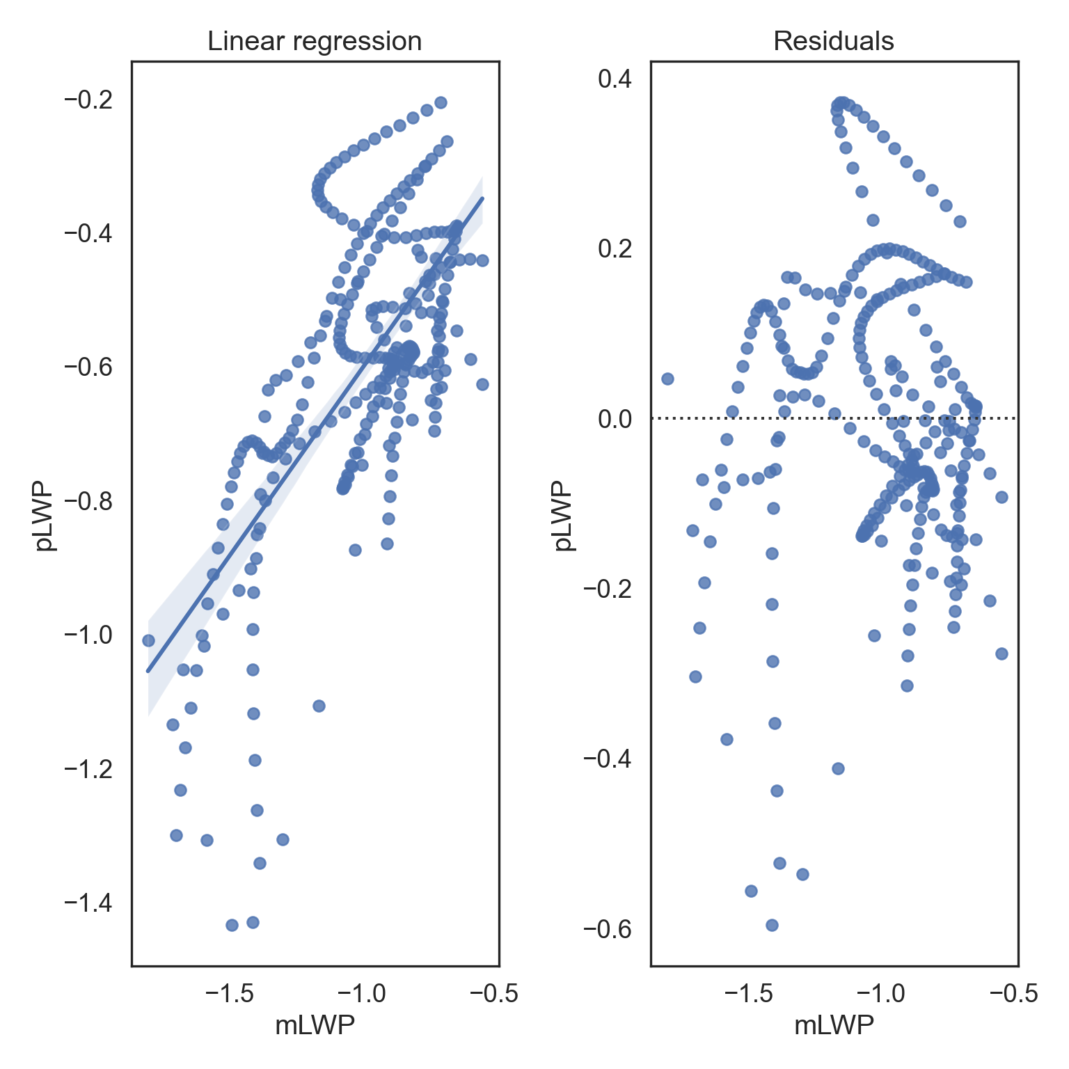

---

Numerical Target Variables: Categorical Variable of Interest

Formula: pLWP (numerical) ~ Group (categorical)

model = ols('pLWP ~ C(Group)', data = data).fit()

sm.stats.anova_lm(model, typ = 2)

             sum_sq     df          F        PR(>F)
C(Group)   2.775293    3.0  22.045408  8.267447e-13
Residual  11.414011  272.0        NaN           NaN

# Increase font and figure size of all seaborn plot elements
sns.set(font_scale = 1.25, rc = {'figure.figsize':(4, 4)})

# Change seaborn plot theme to white
sns.set_style("white")

# Box plot
Group_Box = sns.boxplot(data = data, x = "pLWP", y = "Group", width = 0.3)

# Tweak the visual presentation
Group_Box.set(ylabel = "Group")

# Tight margins
plt.tight_layout()

# Show plot
plt.show()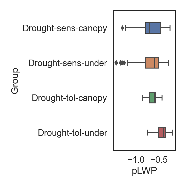

---

Categorical Target Variables: Numerical Variable of Interest

Formula: Group (categorical) ~ pLWP (numerical)

# Grouped describe by one column, stacked 
Groups = data.groupby('Group').describe().unstack(1)

# Print all rows
print(Groups.to_string())

                   Group              
Date        count  Drought-sens-canopy                    147
                   Drought-sens-under                     147
                   Drought-tol-canopy                     147
                   Drought-tol-under                      147
            mean   Drought-sens-canopy    2019-12-16 00:00:00
                   Drought-sens-under     2019-12-16 00:00:00
                   Drought-tol-canopy     2019-12-16 00:00:00
                   Drought-tol-under      2019-12-16 00:00:00
            min    Drought-sens-canopy    2019-10-04 00:00:00
                   Drought-sens-under     2019-10-04 00:00:00
                   Drought-tol-canopy     2019-10-04 00:00:00
                   Drought-tol-under      2019-10-04 00:00:00
            25%    Drought-sens-canopy    2019-11-09 12:00:00
                   Drought-sens-under     2019-11-09 12:00:00
                   Drought-tol-canopy     2019-11-09 12:00:00
                   Drought-tol-under      2019-11-09 12:00:00
            50%    Drought-sens-canopy    2019-12-16 00:00:00
                   Drought-sens-under     2019-12-16 00:00:00
                   Drought-tol-canopy     2019-12-16 00:00:00
                   Drought-tol-under      2019-12-16 00:00:00
            75%    Drought-sens-canopy    2020-01-21 12:00:00
                   Drought-sens-under     2020-01-21 12:00:00
                   Drought-tol-canopy     2020-01-21 12:00:00
                   Drought-tol-under      2020-01-21 12:00:00
            max    Drought-sens-canopy    2020-02-27 00:00:00
                   Drought-sens-under     2020-02-27 00:00:00
                   Drought-tol-canopy     2020-02-27 00:00:00
                   Drought-tol-under      2020-02-27 00:00:00
            std    Drought-sens-canopy                    NaN
                   Drought-sens-under                     NaN
                   Drought-tol-canopy                     NaN
                   Drought-tol-under                      NaN
Sap_Flow    count  Drought-sens-canopy                  120.0
                   Drought-sens-under                   120.0
                   Drought-tol-canopy                   120.0
                   Drought-tol-under                    120.0
            mean   Drought-sens-canopy              85.269653
                   Drought-sens-under                1.448825
                   Drought-tol-canopy                9.074309
                   Drought-tol-under                 4.573516
            min    Drought-sens-canopy               33.37045
                   Drought-sens-under                 0.17263
                   Drought-tol-canopy                 5.90461
                   Drought-tol-under                  2.17178
            25%    Drought-sens-canopy              53.975162
                   Drought-sens-under                0.534165
                   Drought-tol-canopy                 8.11941
                   Drought-tol-under                 4.053346
            50%    Drought-sens-canopy              76.717782
                   Drought-sens-under                1.665492
                   Drought-tol-canopy                9.286552
                   Drought-tol-under                 4.944842
            75%    Drought-sens-canopy              94.068107
                   Drought-sens-under                2.194299
                   Drought-tol-canopy               10.404117
                   Drought-tol-under                 5.139685
            max    Drought-sens-canopy             184.040975
                   Drought-sens-under                2.475989
                   Drought-tol-canopy               10.705455
                   Drought-tol-under                 5.726712
            std    Drought-sens-canopy              41.313962
                   Drought-sens-under                0.803858
                   Drought-tol-canopy                 1.39567
                   Drought-tol-under                  0.90243
TWaterFlux  count  Drought-sens-canopy                  147.0
                   Drought-sens-under                   147.0
                   Drought-tol-canopy                   147.0
                   Drought-tol-under                    147.0
            mean   Drought-sens-canopy              40.404061
                   Drought-sens-under                 0.75177
                   Drought-tol-canopy                4.357234
                   Drought-tol-under                 2.189824
            min    Drought-sens-canopy              12.377738
                   Drought-sens-under                0.101381
                   Drought-tol-canopy                2.036843
                   Drought-tol-under                 0.953906
            25%    Drought-sens-canopy              25.220908
                   Drought-sens-under                 0.27419
                   Drought-tol-canopy                3.601341
                   Drought-tol-under                 1.735003
            50%    Drought-sens-canopy              38.630891
                   Drought-sens-under                0.824875
                   Drought-tol-canopy                4.460778
                   Drought-tol-under                 2.198131
            75%    Drought-sens-canopy              50.096197
                   Drought-sens-under                 1.11289
                   Drought-tol-canopy                5.112844
                   Drought-tol-under                 2.686605
            max    Drought-sens-canopy              96.012719
                   Drought-sens-under                1.801823
                   Drought-tol-canopy                 5.97689
                   Drought-tol-under                 3.654336
            std    Drought-sens-canopy              19.027997
                   Drought-sens-under                0.429073
                   Drought-tol-canopy                0.940353
                   Drought-tol-under                 0.597511
pLWP        count  Drought-sens-canopy                   69.0
                   Drought-sens-under                    69.0
                   Drought-tol-canopy                    69.0
                   Drought-tol-under                     69.0
            mean   Drought-sens-canopy              -0.669932
                   Drought-sens-under               -0.696138
                   Drought-tol-canopy               -0.629909
                   Drought-tol-under                -0.440243
            min    Drought-sens-canopy              -1.299263
                   Drought-sens-under               -1.433333
                   Drought-tol-canopy               -0.863656
                   Drought-tol-under                -0.746667
            25%    Drought-sens-canopy              -0.790573
                   Drought-sens-under                    -0.8
                   Drought-tol-canopy               -0.706479
                   Drought-tol-under                -0.520487
            50%    Drought-sens-canopy              -0.705942
                   Drought-sens-under               -0.592118
                   Drought-tol-canopy               -0.602841
                   Drought-tol-under                -0.406439
            75%    Drought-sens-canopy               -0.47329
                   Drought-sens-under               -0.521217
                   Drought-tol-canopy               -0.571356
                   Drought-tol-under                -0.360789
            max    Drought-sens-canopy              -0.263378
                   Drought-sens-under               -0.299669
                   Drought-tol-canopy               -0.437556
                   Drought-tol-under                -0.205224
            std    Drought-sens-canopy                0.24639
                   Drought-sens-under                0.283935
                   Drought-tol-canopy                0.095571
                   Drought-tol-under                 0.131879
mLWP        count  Drought-sens-canopy                   77.0
                   Drought-sens-under                    77.0
                   Drought-tol-canopy                    77.0
                   Drought-tol-under                     77.0
            mean   Drought-sens-canopy              -1.319148
                   Drought-sens-under               -1.097537
                   Drought-tol-canopy               -0.892554
                   Drought-tol-under                -0.809572
            min    Drought-sens-canopy              -1.812151
                   Drought-sens-under               -1.808333
                   Drought-tol-canopy               -1.073619
                   Drought-tol-under                -1.168716
            25%    Drought-sens-canopy              -1.525563
                   Drought-sens-under               -1.335521
                   Drought-tol-canopy               -0.945841
                   Drought-tol-under                -0.907041
            50%    Drought-sens-canopy              -1.354771
                   Drought-sens-under               -1.054159
                   Drought-tol-canopy               -0.890061
                   Drought-tol-under                -0.735647
            75%    Drought-sens-canopy              -1.111942
                   Drought-sens-under               -0.907564
                   Drought-tol-canopy               -0.828777
                   Drought-tol-under                -0.699087
            max    Drought-sens-canopy              -0.679769
                   Drought-sens-under               -0.546152
                   Drought-tol-canopy               -0.707789
                   Drought-tol-under                -0.545165
            std    Drought-sens-canopy               0.298107
                   Drought-sens-under                0.263522
                   Drought-tol-canopy                0.091729
                   Drought-tol-under                 0.170603

---

Categorical Target Variables: Categorical Variable of Interest

Notably, there is only one categorical variable… Let’s make another:

If \(mLWP > mean(mLWP) + sd(mLWP)\) then Yes, else No.

data1 = data.dropna()
Qual = stat.mean(data1.pLWP + stat.stdev(data1.pLWP))

# Create HighLWP from the age column
def HighLWP_data(data): 
  if data.pLWP >= Qual: return "Yes"
  else: return "No"

# Apply the function to data and create a dataframe
HighLWP = pd.DataFrame(data1.apply(HighLWP_data, axis = 1))

# Name new column
HighLWP.columns = ['HighLWP']

# Concatenate the two dataframes
data1 = pd.concat([data1, HighLWP], axis = 1)

# First six rows of new dataset
data1.head()

        Date                Group    Sap_Flow  ...      pLWP      mLWP  HighLWP
0 2019-10-04  Drought-sens-canopy  184.040975  ... -0.263378 -0.679769      Yes
1 2019-10-04   Drought-sens-under    2.475989  ... -0.299669 -0.761326      Yes
2 2019-10-04   Drought-tol-canopy   10.598949  ... -0.437556 -0.722557       No
3 2019-10-04    Drought-tol-under    4.399854  ... -0.205224 -0.702858      Yes
4 2019-10-05  Drought-sens-canopy  182.905444  ... -0.276928 -0.708261      Yes

[5 rows x 7 columns]

Now we have two categories!

Formula = Group (categorical) ~ HighLWP (categorical)

obs = pd.crosstab(data1.Group, data1.HighLWP)
print(obs)

HighLWP              No  Yes
Group                       
Drought-sens-canopy  58   11
Drought-sens-under   65    4
Drought-tol-canopy   69    0
Drought-tol-under    49   20

# Chi-square test
chi2, p, dof, ex = chi2_contingency(obs, correction = False)
  
# Interpret
alpha = 0.05
  
# Print the interpretation
print('Statistic = %.3f, p = %.3f' % (chi2, p))

Statistic = 30.201, p = 0.000

if p > alpha:
  print('Chi-square value is not greater than critical value (fail to reject H0)')
else:
    print('Chi-square value is greater than critical value (reject H0)')

Chi-square value is greater than critical value (reject H0)

# Increase font and figure size of all seaborn plot elements
sns.set(font_scale = 1.25)

# Change seaborn plot theme to white
sns.set_style("white")

# Count plot of HighLWP grouped by Group 
counts = sns.countplot(data = data1, x = "HighLWP", hue = "Group")

# Tweak the visual presentation
counts.set(ylabel = "Count")

# Tight margins
plt.tight_layout()

# Show plot
plt.show()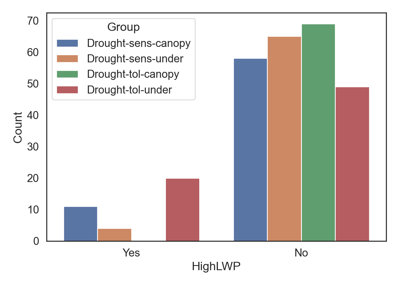

Meredith, Laura, S. Nemiah Ladd, and Christiane Werner. 2021. “Data for "Ecosystem Fluxes During Drought and Recovery in an Experimental Forest".” University of Arizona Research Data Repository. https://doi.org/10.25422/AZU.DATA.14632593.V1.