Reproducing Rise of AI over 8 decades plot

Reproduction of the Our World in Data Plot on the Rise of AI over 8 decades

Author

Affiliation

Dr. Greg Chism

School of Information, University of Arizona

Introduction

This project was conducted to test my ggplot2 skills in reproducing The rise of artificial intelligence over the last 8 decades plot by Our World in Data. The plot has some slight differences based on the data used in my version vs the original.

The original plot is licensed under CC-BY by the authors Charlie Giattino, Edouard Mathieu, and Max Roser. This project is licensed the same.

The data is taken from (Sevilla et al. 2022) – Compute Trends Across Three eras of Machine Learning. Published in arXiv on March 9, 2022. The data are freely available to the public.

The original plot has fewer data points, likely due to additions by the data authors after the original article’s release.

Load required packages

suppressWarnings(library(tidyverse))

# pacman package loader
if(!require(pacman))
  install.packages("pacman")

# Install and load required packages
pacman::p_load(cowplot, # Tools to add an image to a plot
               dlookr, # Exploratory data analysis
               formattable, # HTML formatted outputs
               ggtext, # Text label geoms (particularly richtext)
               here, # For reproducible working directories
               knitr, # Rendering R chunks and RMarkdown
               patchwork, # For adding the image overlayed onto the plot
               png, # To read in an image
               showtext, # To import Google fonts
               tidyverse) # Data wrangling

1

The pacman package is an R package management tool that combines the functionality of base library related functions into intuitively named functions. This line checks if pacman is installed, if not it will be.

2

p_load is a function from pacman package to load packaged from a list. If a package is not installed pacman will both install and load a package.

Dataset Setup

data <- read_csv(here("data", "trendsInLLMs.csv")) |>
  janitor::clean_names() |>
  select(system, publication_date, training_compute_flop, domain) |>
  drop_na() |> 
  mutate(training_compute_flop = as.numeric(training_compute_flop), 
         publication_date = mdy(publication_date),
         publication_date = if_else(publication_date > today(), publication_date - years(100), publication_date),
    domain = case_when(
    domain %in% c("Vision", "Games", "Drawing", "Language") ~ domain,
    domain %in% "Speech" ~ "Language",
    TRUE ~ "Other"
  ),
  domain = factor(domain) |> fct_relevel(c("Vision", "Games", "Drawing", "Language", "Other"))
  )

data |> 
  glimpse()

data |> 
  diagnose() |>
  formattable()

data |> 
  describe() |>
  formattable()

1

The data can be found open source at the following link.

2

Clean the names

3

Select only the relevant columns for analysis.

4

Convert dates that are before 2000 to the 1900s.

5

case_when loop that groups domains.

6

Reorder the factors in the domain column.

7

There are 4 relevant columns, the AI system, the publication data, the training computation FLOP, and the domain.

8

No missing values, data seems clean

9

Summary statistics are as expected for exponential data

Rows: 186
Columns: 4
$ system                <chr> "Falcon 180B", "Swift", "Jais", "Llama 2", "Clau…
$ publication_date      <date> 2023-09-06, 2023-08-30, 2023-08-29, 2023-07-18,…
$ training_compute_flop <dbl> 3.78e+24, 5.34e+16, 3.08e+22, 9.00e+23, 3.30e+25…
$ domain                <fct> Language, Other, Language, Language, Language, L…

variables	types	missing_count	missing_percent	unique_count	unique_rate
system	character	0	0	186	1.00000000
publication_date	Date	0	0	162	0.87096774
training_compute_flop	numeric	0	0	182	0.97849462
domain	factor	0	0	5	0.02688172

described_variables	n	na	mean	sd	se_mean	IQR	skewness	kurtosis	p00	p01	p05	p10	p20	p25	p30	p40	p50	p60	p70	p75	p80	p90	p95	p99	p100
training_compute_flop	186	0	4.342449e+23	2.924188e+24	2.144118e+23	3.24486e+22	9.530386	96.68769	40	592235	1.66e+10	7.69e+13	9.69e+16	1.395e+18	6.82e+18	9.39e+19	8.46e+20	4.42e+21	1.415e+22	3.245e+22	5e+22	3.14e+23	5.695e+23	9.389e+24	3.3e+25

Reproduced plot & code

ggplot2

Original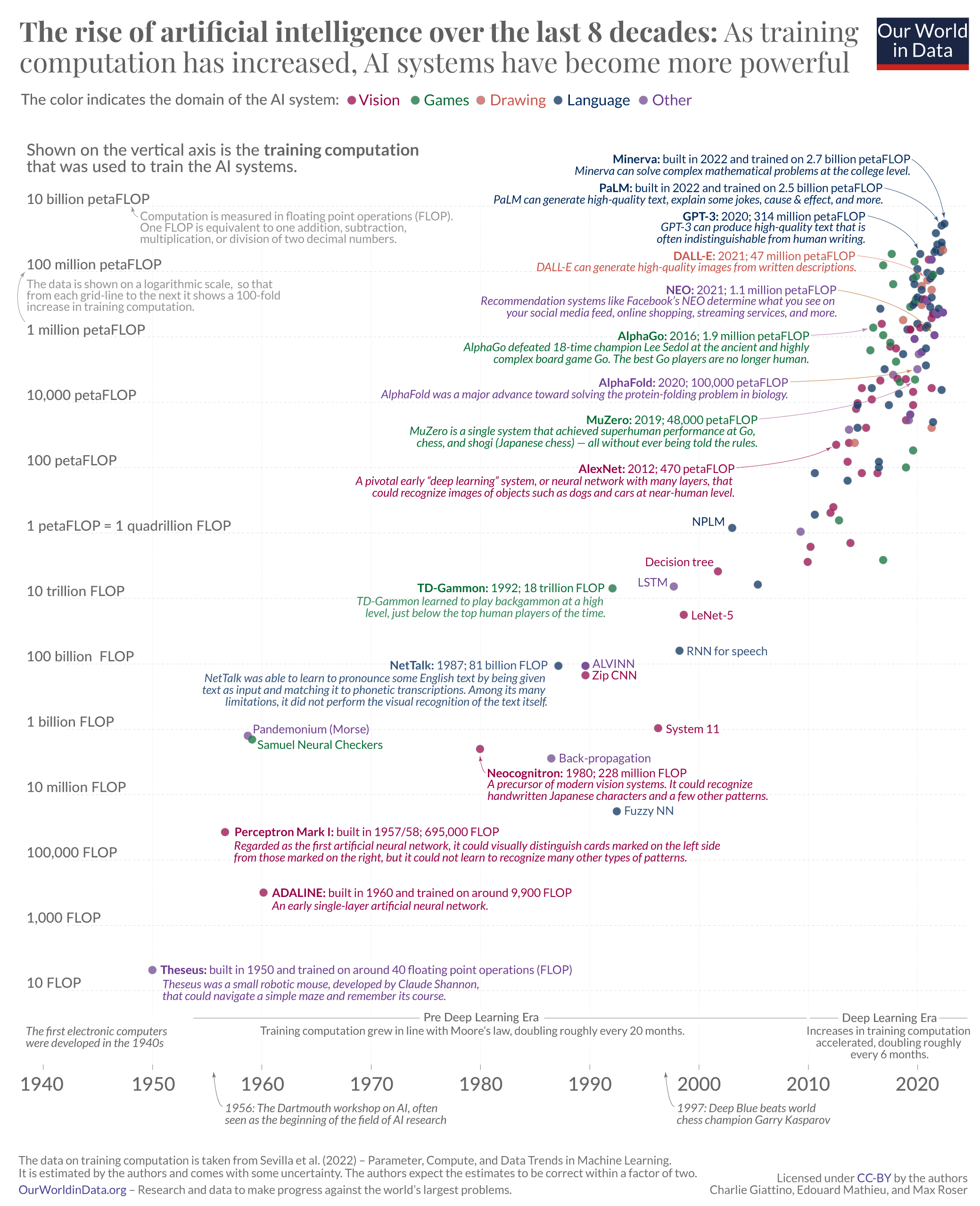

Code

Show the code

# Y-axis breaks
breaks_vals <- as.vector(pretty(log10(data$training_compute_flop), n = 13))

# Y-axis labels
labels_vals <- as.vector(c("0", "10 FLOP", "1,000 FLOP",
                           "100,000 FLOP", "10 million FLOP",
                           "1 billion FLOP", "100 billion FLOP",
                           "10 trillion FLOP", "1 petaFLOP = 1 quadrillion FLOP", 
                           "100 petaFLOP", "10,000 petaFLOP", 
                           "1 million petaFLOP", "100 million petaFLOP", 
                           "10 billion petaFLOP"))

# Add font families 
font_add_google("Playfair Display", "Playfair Display")
font_add_google("Lato", "Lato")
showtext_auto()

# Plot
plot <- data |>
  ggplot(aes(x = publication_date, y = log10(training_compute_flop), color = domain)) +
  geom_segment(x = as.Date("1950-01-01"), xend = as.Date("1950-01-01"),
               y = log10(0.1), yend = log10(1e+25),
               linewidth = 0.05, linetype = 3, color = "#eaeaea") +
  geom_segment(x = as.Date("1960-01-01"), xend = as.Date("1960-01-01"),
               y = log10(0.1), yend = log10(1e+25),
               linewidth = 0.05, linetype = 3, color = "#eaeaea") +
  geom_segment(x = as.Date("1970-01-01"), xend = as.Date("1970-01-01"),
               y = log10(0.1), yend = log10(1e+25),
               linewidth = 0.05, linetype = 3, color = "#eaeaea") +
  geom_segment(x = as.Date("1980-01-01"), xend = as.Date("1980-01-01"),
               y = log10(0.1), yend = log10(1e+25),
               linewidth = 0.05, linetype = 3, color = "#eaeaea") +
  geom_segment(x = as.Date("1990-01-01"), xend = as.Date("1990-01-01"),
               y = log10(0.1), yend = log10(1e+25),
               linewidth = 0.05, linetype = 3, color = "#eaeaea") +
  geom_segment(x = as.Date("2000-01-01"), xend = as.Date("2000-01-01"),
               y = log10(0.1), yend = log10(1e+25),
               linewidth = 0.05, linetype = 3, color = "#eaeaea") +
  geom_segment(x = as.Date("2010-01-01"), xend = as.Date("2010-01-01"),
               y = log10(0.1), yend = log10(1e+25),
               linewidth = 0.05, linetype = 3, color = "#eaeaea") +
  geom_segment(x = as.Date("2020-01-01"), xend = as.Date("2020-01-01"),
               y = log10(0.1), yend = log10(1e+25),
               linewidth = 0.05, linetype = 3, color = "#eaeaea") +
  geom_segment(x = as.Date("1941-01-01"), xend = as.Date("2025-01-01"),
               y = log10(6), yend = log10(6),
               linewidth = 0.05, linetype = 2, color = "#eaeaea") +
  geom_segment(x = as.Date("1941-01-01"), xend = as.Date("2025-01-01"),
               y = log10(6e+2), yend = log10(6e+2),
               linewidth = 0.05, linetype = 2, color = "#eaeaea") +
  geom_segment(x = as.Date("1941-01-01"), xend = as.Date("2025-01-01"),
               y = log10(6e+4), yend = log10(6e+4),
               linewidth = 0.05, linetype = 2, color = "#eaeaea") +
  geom_segment(x = as.Date("1941-01-01"), xend = as.Date("2025-01-01"),
               y = log10(6e+6), yend = log10(6e+6),
               linewidth = 0.05, linetype = 2, color = "#eaeaea") +
  geom_segment(x = as.Date("1941-01-01"), xend = as.Date("2025-01-01"),
               y = log10(6e+8), yend = log10(6e+8),
               linewidth = 0.05, linetype = 2, color = "#eaeaea") +
  geom_segment(x = as.Date("1941-01-01"), xend = as.Date("2025-01-01"),
               y = log10(6e+10), yend = log10(6e+10),
               linewidth = 0.05, linetype = 2, color = "#eaeaea") +
  geom_segment(x = as.Date("1941-01-01"), xend = as.Date("2025-01-01"),
               y = log10(6e+12), yend = log10(6e+12),
               linewidth = 0.05, linetype = 2, color = "#eaeaea") +
  geom_segment(x = as.Date("1941-01-01"), xend = as.Date("2025-01-01"),
               y = log10(6e+14), yend = log10(6e+14),
               linewidth = 0.05, linetype = 2, color = "#eaeaea") +
  geom_segment(x = as.Date("1941-01-01"), xend = as.Date("2025-01-01"),
               y = log10(6e+16), yend = log10(6e+16),
               linewidth = 0.05, linetype = 2, color = "#eaeaea") +
  geom_segment(x = as.Date("1941-01-01"), xend = as.Date("2025-01-01"),
               y = log10(6e+18), yend = log10(6e+18),
               linewidth = 0.05, linetype = 2, color = "#eaeaea") +
  geom_segment(x = as.Date("1941-01-01"), xend = as.Date("2025-01-01"),
               y = log10(6e+20), yend = log10(6e+20),
               linewidth = 0.05, linetype = 2, color = "#eaeaea") +
  geom_segment(x = as.Date("1941-01-01"), xend = as.Date("2025-01-01"),
               y = log10(6e+22), yend = log10(6e+22),
               linewidth = 0.05, linetype = 2, color = "#eaeaea") +
  geom_segment(x = as.Date("1941-01-01"), xend = as.Date("2025-01-01"),
               y = log10(6e+24), yend = log10(6e+24),
               linewidth = 0.05, linetype = 2, color = "#eaeaea") +
  geom_segment(x = as.Date("1953-01-01"), xend = as.Date("2025-01-01"),
               y = log10(2.5), yend = log10(2.5),
               linewidth = 0.03, linetype = 1, color = "#666666") + 
  geom_segment(x = as.Date("1940-01-01"), xend = as.Date("1940-01-01"),
              y = log10(0.09), yend = log10(0.13),
               linewidth = 0.03, linetype = 1, color = "#666666") + 
  geom_segment(x = as.Date("1950-01-01"), xend = as.Date("1950-01-01"),
              y = log10(0.09), yend = log10(0.13),
               linewidth = 0.03, linetype = 1, color = "#666666") +
  geom_segment(x = as.Date("1960-01-01"), xend = as.Date("1960-01-01"),
              y = log10(0.09), yend = log10(0.13),
               linewidth = 0.03, linetype = 1, color = "#666666") +
  geom_segment(x = as.Date("1970-01-01"), xend = as.Date("1970-01-01"),
              y = log10(0.09), yend = log10(0.13),
               linewidth = 0.03, linetype = 1, color = "#666666") +
  geom_segment(x = as.Date("1980-01-01"), xend = as.Date("1980-01-01"),
              y = log10(0.09), yend = log10(0.13),
               linewidth = 0.03, linetype = 1, color = "#666666") +
  geom_segment(x = as.Date("1990-01-01"), xend = as.Date("1990-01-01"),
              y = log10(0.09), yend = log10(0.13),
               linewidth = 0.03, linetype = 1, color = "#666666") +
  geom_segment(x = as.Date("2000-01-01"), xend = as.Date("2000-01-01"),
              y = log10(0.09), yend = log10(0.13),
               linewidth = 0.03, linetype = 1, color = "#666666") +
  geom_segment(x = as.Date("2010-01-01"), xend = as.Date("2010-01-01"),
              y = log10(0.09), yend = log10(0.13),
               linewidth = 0.03, linetype = 1, color = "#666666") +
  geom_segment(x = as.Date("2020-01-01"), xend = as.Date("2020-01-01"),
              y = log10(0.09), yend = log10(0.13),
               linewidth = 0.03, linetype = 1, color = "#666666") +
  geom_point(alpha = 0.85) +
  geom_curve(
    aes(x = as.Date("1980-04-01"), y = log10(1.75e+07),
        xend = as.Date("1980-04-01"), yend = log10(1.5e+08)),
    curvature = -0.2,
    arrow = arrow(length = unit(0.005, "npc"), type = "closed"),
    color = "#B4477A",
    linewidth = 0.1
  ) +
  geom_curve(
    aes(x = as.Date("2003-07-15"), y = log10(5e+16),
        xend = as.Date("2012-02-27"), yend = log10(4.5e+17)),
    curvature = 0.2,
    arrow = arrow(length = unit(0.005, "npc"), type = "closed"),
    color = "#B4477A",
    linewidth = 0.1
  ) +
  geom_curve(
    aes(x = as.Date("2006-06-15"), y = log10(1.2e+18),
        xend = as.Date("2019-06-19"), yend = log10(4e+19)),
    curvature = 0.2,
    arrow = arrow(length = unit(0.005, "npc"), type = "closed"),
    color = "#4B946C",
    linewidth = 0.1
    ) +
  geom_curve(
    aes(x = as.Date("2009-06-15"), y = log10(1.5e+19),
        xend = as.Date("2019-07-15"), yend = log10(9e+19)),
    curvature = 0.2,
    arrow = arrow(length = unit(0.005, "npc"), type = "closed"),
    color = "#9674B0",
    linewidth = 0.1
  ) +
  geom_curve(
    aes(x = as.Date("2009-06-15"), y = log10(4.5e+20),
        xend = as.Date("2015-06-27"), yend = log10(1.33e+21)),
    curvature = 0.2,
    arrow = arrow(length = unit(0.005, "npc"), type = "closed"),
    color = "#4B946C",
    linewidth = 0.1
    ) +
  geom_curve(
    aes(x = as.Date("2010-02-15"), y = log10(1.5e+22),
        xend = as.Date("2021-03-21"), yend = log10(7.90e+21)),
    curvature = -0.1,
    arrow = arrow(length = unit(0.005, "npc"), type = "closed"),
    color = "#476589",
    linewidth = 0.1
    ) +
  geom_curve(
    aes(x = as.Date("2011-03-15"), y = log10(1.5e+23),
        xend = as.Date("2021-01-05"), yend = log10(4.7e+22)),
    curvature = -0.1,
    arrow = arrow(length = unit(0.005, "npc"), type = "closed"),
    color = "#D8847C",
    linewidth = 0.1
    ) +
  geom_curve(
    aes(x = as.Date("2012-06-15"), y = log10(2.5e+24),
        xend = as.Date("2020-01-28"), yend = log10(4e+23)),
    curvature = -0.1,
    arrow = arrow(length = unit(0.005, "npc"), type = "closed"),
    color = "#476589",
    linewidth = 0.1
    ) +
  geom_curve(
    aes(x = as.Date("2014-12-15"), y = log10(3e+25),
        xend = as.Date("2021-06-04"), yend = log10(3e+24)),
    curvature = -0.1,
    arrow = arrow(length = unit(0.005, "npc"), type = "closed"),
    color = "#476589",
    linewidth = 0.1
    ) +
  geom_curve(
    aes(x = as.Date("2016-12-15"), y = log10(3e+26),
        xend = as.Date("2021-12-04"), yend = log10(5e+24)),
    curvature = -0.1,
    arrow = arrow(length = unit(0.005, "npc"), type = "closed"),
    color = "#476589",
    linewidth = 0.1
    ) +
  geom_curve(
    aes(x = as.Date("1938-01-01"), y = log10(1e+21),
        xend = as.Date("1938-01-01"), yend = log10(1e+23)),
    curvature = -0.3,
    arrow = arrow(length = unit(0.005, "npc"), type = "closed"),
    color = "#929292",
    linewidth = 0.1
    ) +
  geom_curve( 
    aes(x = as.Date("1948-08-01"), y = log10(2e+24),
        xend = as.Date("1948-03-01"), yend = log10(5e+24)),
    curvature = -0.15,
    arrow = arrow(length = unit(0.005, "npc"), type = "closed"),
    color = "#929292",
    linewidth = 0.1
    ) +
  geom_curve(
    aes(x = as.Date("1957-06-01"), y = log(0.1),
        xend = as.Date("1956-01-01"), yend = log10(0.05)),
    curvature = -0.15,
    arrow = arrow(length = unit(0.005, "npc"), type = "closed"),
    color = "#929292",
    linewidth = 0.1
    ) +
  geom_curve(
    aes(x = as.Date("1998-06-01"), y = log(0.1),
        xend = as.Date("1997-01-01"), yend = log10(0.05)),
    curvature = -0.15,
    arrow = arrow(length = unit(0.005, "npc"), type = "closed"),
    color = "#929292",
    linewidth = 0.1
    ) +
  annotate(geom = "richtext",
           x = as.Date("1950-07-05"), y = log10(40), 
           label = "<span style='color:#9674B0;'><b>Theseus:</b> built in 1950 and trained on around 40 floating point operations (FLOP)<br><i>Theseus was a small robotic mouse, developed by Claude Shannon,<br>that could navigate a simple maze and remember its course.</i></span>",
           size = 3,
           family = "Open Sans",
           fill = NA,
           label.color = NA,
           hjust = 0,
           vjust = 0.5) +
  annotate(geom = "richtext", 
           x = as.Date("1960-06-30"), y = log10(9900), 
           label = "<span style='color:#B4477A;'><b>ADALINE:</b> built in 1960 and trained on aroiund 9,900 FLOP<br><i>An early single-layer artificial neural network.</i></span>",
           size = 3,
           family = "Open Sans",
           fill = NA,
           label.color = NA,
           hjust = 0,
           vjust = 0.75) +
  annotate(geom = "richtext", 
           x = as.Date("1957-01-01"), y = log10(695000), 
           label = "<span style='color:#B4477A;'><b>Perceptron Mark I:</b> built in 1957/58, 695,000 FLOP<br><i>Regarded as the first artificial neural network, it could visually distinguish cards marked on the left side<br>from those marked on the right, but it could not learn to recognize many other patterns.</i></span>",
           size = 3,
           family = "Open Sans",
           fill = NA,
           label.color = NA,
           hjust = 0,
           vjust = 0.8) +
  annotate(geom = "richtext", 
           x = as.Date("1992-09-01"), y = log10(1400000000), 
           label = "<span style='color:#476589;'>Fuzzy NN</span>",
           size = 3,
           family = "Open Sans",
           fill = NA,
           label.color = NA,
           hjust = 0,
           vjust = 0.55) +
  annotate(geom = "richtext", 
           x = as.Date("1980-04-01"), y = log10(0.5e+08), 
           label = "<span style='color:#B4477A;'><b>Neocognitron:</b> built in 1980, 228 million FLOP<br><i>A precursor of modern vision systems. It could recognize<br>handwritten Japanese characters and a few other patterns.</i></span>",
           size = 3,
           family = "Open Sans",
           fill = NA,
           label.color = NA,
           hjust = 0,
           vjust = 0.8) +
  annotate(geom = "richtext", 
           x = as.Date("1959-02-01"), y = log10(6e+08), 
           label = "<span style='color:#9674B0;'>Pandemonium (morse)</span>",
           size = 3,
           family = "Open Sans",
           fill = NA,
           label.color = NA,
           hjust = 0.05,
           vjust = 0.15) +
  annotate(geom = "richtext", 
           x = as.Date("1959-10-01"), y = log10(1.28e+08), 
           label = "<span style='color:#4B946C;'>Samuel Neural Checkers</span>",
           size = 3,
           family = "Open Sans",
           fill = NA,
           label.color = NA,
           hjust = 0.05,
           vjust = 0) +
  annotate(geom = "richtext", 
           x = as.Date("1987-03-06"), y = log10(8e+10), 
           label = "<span style='color:#476589; text-align:center;'><b>NetTalk:</b> 1987; 81 billion FLOP<br><i>NetTalk was able to learn to pronounce some English text by given<br>text as input and matching it to phonetic transcriptions. Among its many<br>limitations, it did not perform the visual recognition of the text itself.</i></span>",
           size = 3,
           family = "Open Sans",
           fill = NA,
           label.color = NA,
           hjust = 1,
           vjust = 0.8) +
  annotate(geom = "richtext", 
           x = as.Date("1989-12-01"), y = log10(8.12e+10), 
           label = "<span style='color:#9674B0;'>ALVINN</span>",
           size = 3,
           family = "Open Sans",
           fill = NA,
           label.color = NA,
           hjust = 0,
           vjust = 0.55) +
  annotate(geom = "richtext", 
           x = as.Date("1989-12-01"), y = log10(4.34e+10), 
           label = "<span style='color:#B4477A;'>Zip CNN</span>",
           size = 3,
           family = "Open Sans",
           fill = NA,
           label.color = NA,
           hjust = 0,
           vjust = 0.55) +
  annotate(geom = "richtext", 
           x = as.Date("1996-06-18"), y = log10(1.29e+10), 
           label = "<span style='color:#B4477A;'>System 11</span>",
           size = 3,
           family = "Open Sans",
           fill = NA,
           label.color = NA,
           hjust = 0,
           vjust = 0.55) +
  annotate(geom = "richtext", 
           x = as.Date("1986-10-01"), y = log10(1.24e+08), 
           label = "<span style='color:#9674B0;'>Back-propagation</span>",
           size = 3,
           family = "Open Sans",
           fill = NA,
           label.color = NA,
           hjust = 0.1,
           vjust = 0) +
  annotate(geom = "richtext", 
           x = as.Date("1989-01-01"), y = log10(1.2e+08), 
           label = "<span style='color:#9674B0;'>Innervator</span>",
           size = 3,
           family = "Open Sans",
           fill = NA,
           label.color = NA,
           hjust = 0,
           vjust = 0.55) +
    annotate(geom = "richtext", 
           x = as.Date("1998-05-15"), y = log10(2.27e+11), 
           label = "<span style='color:#476589;'>RNN for speech</span>",
           size = 3,
           family = "Open Sans",
           fill = NA,
           label.color = NA,
           hjust = 0,
           vjust = 0.8) +
  annotate(geom = "richtext", 
           x = as.Date("1992-05-01"), y = log10(1.82e+13), 
           label = "<span style='color:#4B946C; text-align:center;'><b>TD-Gammon:</b> 1992; 18 trillion FLOP<br><i>TD-Gammon learned to play backgammon at a high<br>level, just below the top human players of the time.</i></span>",
           size = 3,
           family = "Open Sans",
           fill = NA,
           label.color = NA,
           hjust = 1,
           vjust = 0.8) +
  annotate(geom = "richtext", 
           x = as.Date("1998-11-01"), y = log10(2.81e+12), 
           label = "<span style='color:#B4477A;'>LeNet-5</span>",
           size = 3,
           family = "Open Sans",
           fill = NA,
           label.color = NA,
           hjust = 0,
           vjust = 0.55) +
  annotate(geom = "richtext", 
           x = as.Date("1997-11-15"), y = log10(2.10e+13), 
           label = "<span style='color:#476589;'>LSTM</span>",
           size = 3,
           family = "Open Sans",
           fill = NA,
           label.color = NA,
           hjust = 0,
           vjust = 0.55) +
  annotate(geom = "richtext", 
           x = as.Date("2001-12-08"), y = log10(6.3e+13), 
           label = "<span style='color:#B4477A;'>Decision tree</span>",
           size = 3,
           family = "Open Sans",
           fill = NA,
           label.color = NA,
           hjust = 1,
           vjust = 0.15) +
    annotate(geom = "richtext", 
           x = as.Date("2003-03-15"), y = log10(1.3e+15), 
           label = "<span style='color:#476589;'>NPLM</span>",
           size = 3,
           family = "Open Sans",
           fill = NA,
           label.color = NA,
           hjust = 1,
           vjust = 0.15) +
  annotate(geom = "richtext", 
           x = as.Date("2003-07-15"), y = log10(8e+15), 
           label = "<span style='color:#B4477A; text-align:center;'><b>AlexNet:</b> 2012; 470 petaFLOP<br><i>A pivotal early deep learning system, or neural network with many layers, that<br>could recognize images of objects such as dogs and cars at near-human level.</i></span>",
           size = 3,
           family = "Open Sans",
           fill = NA,
           label.color = NA,
           hjust = 1,
           vjust = 0.15) +
  annotate(geom = "richtext", 
           x = as.Date("2006-06-15"), y = log10(2e+17), 
           label = "<span style='color:#4B946C; text-align:center;'><b>MuZero:</b> 2019; 48,000 petaFLOP<br><i>MuZero is a single system that achieved superhuman performance at Go<br>chess, and shogi (Japanese chess) - all without ever being told the rules.</i></span>",
           size = 3,
           family = "Open Sans",
           fill = NA,
           label.color = NA,
           hjust = 1,
           vjust = 0.15) +
  annotate(geom = "richtext", 
           x = as.Date("2009-06-15"), y = log10(5e+18), 
           label = "<span style='color:#9674B0; text-align:center;'><b>AlphaFold:</b> 2020; 100,000 petaFLOP<br><i>AlphaFold was a major advance toward solving the protein-folding problem in biology.</i></span>",
           size = 3,
           family = "Open Sans",
           fill = NA,
           label.color = NA,
           hjust = 1,
           vjust = 0.15) +
  annotate(geom = "richtext", 
           x = as.Date("2010-06-15"), y = log10(2e+21),
           label = "<span style='color:#476589; text-align:center;'><b>NEO:</b> 2021; 1.1 million petaFLOP<br><i>Recommendation systems like Facebook&apos;s NEO determine what you see on<br>your social media feed, online shopping, streaming services, and more.</i></span>",
           size = 3,
           family = "Open Sans",
           fill = NA,
           label.color = NA,
           hjust = 1,
           vjust = 0.15) +
  annotate(geom = "richtext", 
           x = as.Date("2009-06-15"), y = log10(7e+19),
           label = "<span style='color:#4B946C; text-align:center;'><b>AlphaGo:</b> 2016; 1.9 million petaFLOP<br><i>AlphaGo defeated 18-time champion Lee Sedol at the ancient and highly<br>complex board game Go. The best Go players are no longer human.</i></span>",
           size = 3,
           family = "Open Sans",
           fill = NA,
           label.color = NA,
           hjust = 1,
           vjust = 0.15) +
  annotate(geom = "richtext", 
           x = as.Date("2011-06-15"), y = log10(5e+22),
           label = "<span style='color:#D8847C; text-align:center;'><b>DALL-E:</b> 2021; 47 million petaFLOP<br><i>DALL-E can generate high-quality images from writteen descriptions.</i></span>",
           size = 3,
           family = "Open Sans",
           fill = NA,
           label.color = NA,
           hjust = 1,
           vjust = 0.15) +
  annotate(geom = "richtext", 
           x = as.Date("2012-06-15"), y = log10(5e+23),
           label = "<span style='color:#476589; text-align:center;'><b>GPT-3:</b> 2021; 314 million petaFLOP<br><i>GPT-3 can produce high-quality text that is<br>often indistinguishable from human writing.</i></span>",
           size = 3,
           family = "Open Sans",
           fill = NA,
           label.color = NA,
           hjust = 1,
           vjust = 0.15) +
  annotate(geom = "richtext", 
           x = as.Date("2014-12-15"), y = log10(1e+25),
           label = "<span style='color:#476589; text-align:center;'><b>PaLM:</b> 2022; built in 2022 and trained on 2.5 petaFLOP<br><i>PaLM can generate high-quality text, explain some jokes, cause & effect, and more.</i></span>",
           size = 3,
           family = "Open Sans",
           fill = NA,
           label.color = NA,
           hjust = 1,
           vjust = 0.15) +
  annotate(geom = "richtext", 
           x = as.Date("2016-12-15"), y = log10(1e+26),
           label = "<span style='color:#476589; text-align:center;'><b>Minerva:</b> 2022; built in 2022 and trained on 2.7 petaFLOP<br><i>Minerva can solve complex mathematical problems at the college level.</i></span>",
           size = 3,
           family = "Open Sans",
           fill = NA,
           label.color = NA,
           hjust = 1,
           vjust = 0.15) +
    annotate(geom = "richtext",
           x = as.Date("1938-01-01"), y = log10(5e+21),
           label = "<span style='color:#929292; text-align:center;'>The data is shown on a logarithmic scale, so that<br>from each grid-line to the next it shows a 100-fold<br>increase in training computation.</span>",
           size = 2.75,
           family = "Open Sans",
           fill = NA,
           label.color = NA,
           hjust = 0,
           vjust = 0.25) +
  annotate(geom = "richtext", 
           x = as.Date("1948-06-01"), y = log10(3e+23),
           label = "<span style='color:#929292; text-align:center;'>Computation is measured in floating point operations (FLOP).<br>One FLOP is equivalent to one addition, subtraction,<br>multiplication, or division of two decimal numbers.</span>",
           size = 2.75,
           family = "Open Sans",
           fill = NA,
           label.color = NA,
           hjust = 0,
           vjust = 0.15) +
  annotate(geom = "richtext", 
           x = as.Date("1938-01-01"), y = log10(7e+25),
           label = "<span style='color:#666666; text-align:center;'>Shown on the vertical axis in the <b>training computation</b><br>that was used to train the AI systems.</span>",
           size = 3.75,
           fill = NA,
           label.color = NA,
           hjust = 0,
           vjust = 0.15) +
  annotate(geom = "richtext",
           x = as.Date("1938-01-01"), y = log10(0.6),
           label = "<span style='color:#666666;'><i>The first electronic computers<br>were developed in the 1940s</i></span>", 
           hjust = 0,
           size = 2.85,
           fill = NA,
           label.color = NA) +
  annotate(geom = "richtext",
           x = as.Date("1957-01-01"), y = log(0.08),
           label = "<span style='color:#666666;'><i>1956: The Dartmouth workshop on AI, often<br>seen as the beginning of the field of AI research</i></span>",
           hjust = 0,
           size = 3,
           family = "Open Sans",
           fill = NA,
           label.color = NA) +
  annotate(geom = "richtext",
           x = as.Date("1998-01-01"), y = log(0.08),
           label = "<span style='color:#666666;'><i>1997: Deep Blue beats world<br>chess champion Garry Kasparov</i></span>",
           hjust = 0,
           size = 3,
           family = "Open Sans",
           fill = NA,
           label.color = NA) +
  annotate(geom = "richtext",
           x = as.Date("1938-01-01"), y = log10(0.00003),
           label = "<span style='color:#666666; text-align:center;'>The data on training computation is taken from Sevilla et al. (2022) - Parameter, Compute, and Data Trends in Machine Learning.<br>It is estimated by the authors and comes with some uncertainty. The authors expect the estimated to be correct within a factor or two.<br></span><span style='color:#524E98;'>OurWorldInData.org </span><span style='color:#666666;'>- Research and data to make progress against the world&apos;s largest problems.",
           size = 2.3,
           family = "Open Sans",
           fill = NA,
           label.color = NA,
           hjust = 0,
           vjust = 0.15) +
  annotate(geom = "richtext", 
           x = as.Date("2022-01-01"), y = log10(0.00005),
           label = "<span style='color:#666666; text-align:center;'>Licensed under </span><span style='color:#524E98;'>CC-BY  </span><span style='color:#666666;'>by the authors<br>Charlie Giattino, Edouard Mathieu, and Max Roser.",
           size = 2.3,
           family = "Open Sans",
           fill = NA,
           label.color = NA,
           hjust = 1,
           vjust = 0.1) +
  annotate(geom = "richtext",
           x = as.Date("1938-01-01"), y = log10(10),
           label = "<span style='color:#666666;'>10 FLOP</span>", 
           hjust = 0,
           size = 3.25,
           fill = NA,
           label.color = NA) +
  annotate(geom = "richtext",
           x = as.Date("1938-01-01"), y = log10(1000),
           label = "<span style='color:#666666;'>1,000 FLOP</span>", 
           hjust = 0,
           size = 3.25,
           family = "Open Sans",
           fill = NA,
           label.color = NA) +
  annotate(geom = "richtext",
           x = as.Date("1938-01-01"), y = log10(1e+5),
           label = "<span style='color:#666666;'>100,000 FLOP</span>", 
           hjust = 0,
           size = 3.25,
           family = "Open Sans",
           fill = NA,
           label.color = NA) +
  annotate(geom = "richtext",
           x = as.Date("1938-01-01"), y = log10(1e+7),
           label = "<span style='color:#666666;'>10 million FLOP</span>", 
           hjust = 0,
           size = 3.25,
           family = "Open Sans",
           fill = NA,
           label.color = NA) +
  annotate(geom = "richtext",
           x = as.Date("1938-01-01"), y = log10(1e+9),
           label = "<span style='color:#666666;'>1 billion FLOP</span>", 
           hjust = 0,
           size = 3.25,
           family = "Open Sans",
           fill = NA,
           label.color = NA) +
  annotate(geom = "richtext",
           x = as.Date("1938-01-01"), y = log10(1e+11),
           label = "<span style='color:#666666;'>100 billion FLOP</span>", 
           hjust = 0,
           size = 3.25,
           family = "Open Sans",
           fill = NA,
           label.color = NA) +
  annotate(geom = "richtext",
           x = as.Date("1938-01-01"), y = log10(1e+13),
           label = "<span style='color:#666666;'>10 trillion FLOP</span>", 
           hjust = 0,
           size = 3.25,
           family = "Open Sans",
           fill = NA,
           label.color = NA) +
  annotate(geom = "richtext",
           x = as.Date("1938-01-01"), y = log10(1e+15),
           label = "<span style='color:#666666;'>1 petaFLOP = 1 quadrillion FLOP</span>", 
           hjust = 0,
           size = 3.25,
           family = "Open Sans",
           fill = NA,
           label.color = NA) +
  annotate(geom = "richtext",
           x = as.Date("1938-01-01"), y = log10(1e+17),
           label = "<span style='color:#666666;'>100 petaFLOP</span>", 
           hjust = 0,
           size = 3.25,
           family = "Open Sans",
           fill = NA,
           label.color = NA) +
  annotate(geom = "richtext",
           x = as.Date("1938-01-01"), y = log10(1e+19),
           label = "<span style='color:#666666;'>10,000 petaFLOP</span>", 
           hjust = 0,
           size = 3.25,
           family = "Open Sans",
           fill = NA,
           label.color = NA) +
  annotate(geom = "richtext",
           x = as.Date("1938-01-01"), y = log10(1e+21),
           label = "<span style='color:#666666;'>1 million petaFLOP</span>", 
           hjust = 0,
           size = 3.25,
           family = "Open Sans",
           fill = NA,
           label.color = NA) +
  annotate(geom = "richtext",
           x = as.Date("1938-01-01"), y = log10(1e+23),
           label = "<span style='color:#666666;'>100 million petaFLOP</span>", 
           hjust = 0,
           size = 3.25,
           family = "Open Sans",
           fill = NA,
           label.color = NA) +
  annotate(geom = "richtext",
           x = as.Date("1938-01-01"), y = log10(1e+25),
           label = "<span style='color:#666666;'>10 billion petaFLOP</span>", 
           hjust = 0,
           size = 3.25,
           family = "Open Sans",
           fill = NA,
           label.color = NA) +
  annotate(geom = "richtext",
           x = as.Date("2020-01-01"), y = log10(0.03),
           label = "<span style='color:#666666;'>2020</span>", 
           hjust = 0.5,
           size = 4.5,
           family = "Open Sans",
           fill = NA,
           label.color = NA) +
  annotate(geom = "richtext",
           x = as.Date("2010-01-01"), y = log10(0.03),
           label = "<span style='color:#666666;'>2010</span>", 
           hjust = 0.5,
           size = 4.5,
           family = "Open Sans",
           fill = NA,
           label.color = NA) +
  annotate(geom = "richtext",
           x = as.Date("2000-01-01"), y = log10(0.03),
           label = "<span style='color:#666666;'>2000</span>", 
           hjust = 0.5,
           size = 4.5,
           family = "Open Sans",
           fill = NA,
           label.color = NA) +
  annotate(geom = "richtext",
           x = as.Date("1990-01-01"), y = log10(0.03),
           label = "<span style='color:#666666;'>1990</span>", 
           hjust = 0.5,
           size = 4.5,
           family = "Open Sans",
           fill = NA,
           label.color = NA) +
  annotate(geom = "richtext",
           x = as.Date("1980-01-01"), y = log10(0.03),
           label = "<span style='color:#666666;'>1980</span>", 
           hjust = 0.5,
           size = 4.5,
           family = "Open Sans",
           fill = NA,
           label.color = NA) +
  annotate(geom = "richtext",
           x = as.Date("1970-01-01"), y = log10(0.03),
           label = "<span style='color:#666666;'>1970</span>", 
           hjust = 0.5,
           size = 4.5,
           family = "Open Sans",
           fill = NA,
           label.color = NA) +
  annotate(geom = "richtext",
           x = as.Date("1960-01-01"), y = log10(0.03),
           label = "<span style='color:#666666;'>1960</span>", 
           hjust = 0.5,
           size = 4.5,
           family = "Open Sans",
           fill = NA,
           label.color = NA) +
  annotate(geom = "richtext",
           x = as.Date("1950-01-01"), y = log10(0.03),
           label = "<span style='color:#666666;'>1950</span>", 
           hjust = 0.5,
           size = 4.5,
           family = "Open Sans",
           fill = NA,
           label.color = NA) +
  annotate(geom = "richtext",
           x = as.Date("1940-01-01"), y = log10(0.03),
           label = "<span style='color:#666666;'>1940</span>", 
           hjust = 0.5,
           size = 4.5,
           family = "Open Sans",
           fill = NA,
           label.color = NA) +
  annotate(geom = "richtext",
           x = as.Date("1980-01-01"), y = log10(2.3),
           label = "<span style='color:#666666;'>Pre Deep Learning Era</span>", 
           hjust = 0.5,
           size = 3,
           family = "Open Sans",
           fill = "white",
           label.color = NA) +
  annotate(geom = "richtext",
           x = as.Date("1980-01-01"), y = log10(0.9),
           label = "<span style='color:#666666;'>Training computation grew in line with Moore&apos;s law, doubling every 20 months</span>", 
           hjust = 0.5,
           size = 2.85,
           family = "Open Sans",
           fill = NA, 
           lineheight = 0.5, 
           label.color = NA) +
  annotate(geom = "richtext",
           x = as.Date("2018-01-01"), y = log10(2.3),
           label = "<span style='color:#666666;'>Deep Learning Era</span>", 
           hjust = 0.5,
           size = 3,
           family = "Open Sans",
           fill = "white",
           label.color = NA) +
  annotate(geom = "richtext",
           x = as.Date("2018-01-01"), y = log10(0.4),
           label = "<span style='color:#666666;'>Increases in training computation<br>accelerated, doubling roughlt<br>every 6 months</span>", 
           hjust = 0.5,
           size = 2.85,
           family = "Open Sans",
           fill = NA, 
           label.color = NA) +
  scale_x_date(breaks = seq(as.Date("1940-01-01"), as.Date("2020-01-01"), by = "10 years"),
               date_labels = "%Y") +
  scale_y_continuous(breaks = breaks_vals, labels = labels_vals) +
  scale_color_manual(values = c("#B4477A", "#4B946C", "#D8847C", "#476589", "#9674B0"),
                     labels = c("<span style='color:#B4477A;'>Vision</span>",
                                "<span style='color:#4B946C;'>Games</span>",
                                "<span style='color:#D8847C;'>Drawing</span>",
                                "<span style='color:#476589;'>Language</span>",
                                "<span style='color:#9674B0;'>Other</span>")) +
  theme_void(base_size = 11, base_family = "Open Sans") +
  labs(x = NULL,
       y = NULL,
       color = "The color indicates the domain of the AI system:",
       title = "<span style='color:#666666;'><b>The rise of artificial intelligence over the last 8 decades:</b> As training<br>computation has increased, AI systems have become more powerful</span>"
       ) + 
  guides(color = guide_legend(override.aes = list(alpha = 1))) +
  theme(legend.position = c(0.3675, 0.985),
        legend.direction = "horizontal",
        legend.spacing.x = unit(-0.1,'cm'),
        legend.title = element_markdown(family = "Open Sans", size = 10, color = "#666666"),
        legend.text = element_markdown(family = "Open Sans", size = 10),
        plot.title = element_markdown(hjust = 0.2275, vjust = 0.99, size = 18.5, family = "Playfair Display"),
        plot.title.position = "plot",
        plot.margin = margin(t = 0, r = -10, b = -10, l = -10),
        axis.text = element_blank())

logo <- png::readPNG(here("images", "ourWorldDataLogo.png"), native = TRUE)

plot +
  inset_element(p = logo,
                left = 0.865,
                bottom = 0.89,
                right = 0.95,
                top = 1.15,
                on_top = FALSE)

1

List of breaks for the y-axis (13 in total)

2

Labels for breaks for the y-axis

3

Add the necessary Google Fonts (Playfair Display for the title, Open Sans for all other text)

4

ggplot with publication date on the x-axis, log10 transformed training computation FLOP on the y-axis, color is the domain

5

Begins a series of geom_segment lines that create the background grid.

6

Creates the dark line from 1953-01-01 to 2025-01-01, at log10(2.5) on the y-axis

7

Begins the geom_segments that make up the x-axis ticks

8

Adds scatterplot points, with alpha = 0.85 (they will be colored by domain)

9

Begins the geom_curve arrows that point to individual AI systems from their label

10

Begins grey geom_curve arrows that point to axis point explanations

11

Begins annotations for individual AI systems of significants

12

Begins annotations for significant events or information on the x-axis

13

Begins annotations for significant events or information on the y-axis

14

Begins annotations for the bottom captions

15

Begins y-axis label annotations

16

Begins x-axis label annotations

17

Begins annotations for text overlayed onto the dark geom_segment spanning horizontally under 10 FLOP

18

Scale date x-axis from 1940 - 2020 by 10 years, labeled by year (technically redundant now…)

19

Scale continuous numerical y-axis by the pre-defined breaks and labels

20

Manually scale the colors for each domain, specifically values and labels

21

Set theme_void as the underlying theme, make the base font size 11 and family Open Sans

22

Remove axes labels

23

Set the color legend title

24

Set the plot title (its “richtext”)

25

Move the legend to start the title at the left margin of the plot

26

Set the legend to a horizontal direction

27

Move the legend values for each color-domain closer

28

Set the legend title as an element_markdown, which allows us to use HTML and CSS code in “rich text”

29

Set the legend text as an element_markdown, which allows us to use HTML and CSS code in “rich text”

30

Set the plot title as an element_markdown, which allows us to use HTML and CSS code in “rich text”, position it to the left margin, set the font family to Playfair Display

31

Places the title inside the plot area, just above the main content

32

Set margins, top and right are the same, bottom is reduced by 1 grid unit and left is added by 10 grid units

33

Remove axis text

34

Read in the Our World In Data logo

35

Add the logo on top of the plot, but under plot elements other than the background

References

Sevilla, Jaime, Lennart Heim, Anson Ho, Tamay Besiroglu, Marius Hobbhahn, and Pablo Villalobos. 2022. “Compute Trends Across Three Eras of Machine Learning.” https://doi.org/10.48550/ARXIV.2202.05924.