# Data Manipulation and Analysis
import pandas as pd
import numpy as np

# Data Visualization
import seaborn as sns
import matplotlib.pyplot as plt

# Machine Learning
from sklearn.decomposition import PCA
from sklearn.impute import SimpleImputer
from sklearn.preprocessing import StandardScaler, OneHotEncoder

# Statistical Analysis
import statsmodels.api as sm
import scipy.stats as stats

# Increase font size of all Seaborn plot elements
sns.set(font_scale=1.25)

# Set Seaborn theme
sns.set_theme(style="whitegrid", palette="colorblind")PCA + Clustering
INFO Data Visualization and Analysis - Week 5
UArizona School of Information
Setup
Data Preprocessing
Data preprocessing can refer to manipulation, filtration or augmentation of data before it is analyzed, and is often an important step in the data analysis process.
Datasets
Human Freedom Index
The Human Freedom Index is a report that attempts to summarize the idea of “freedom” through variables for many countries around the globe.
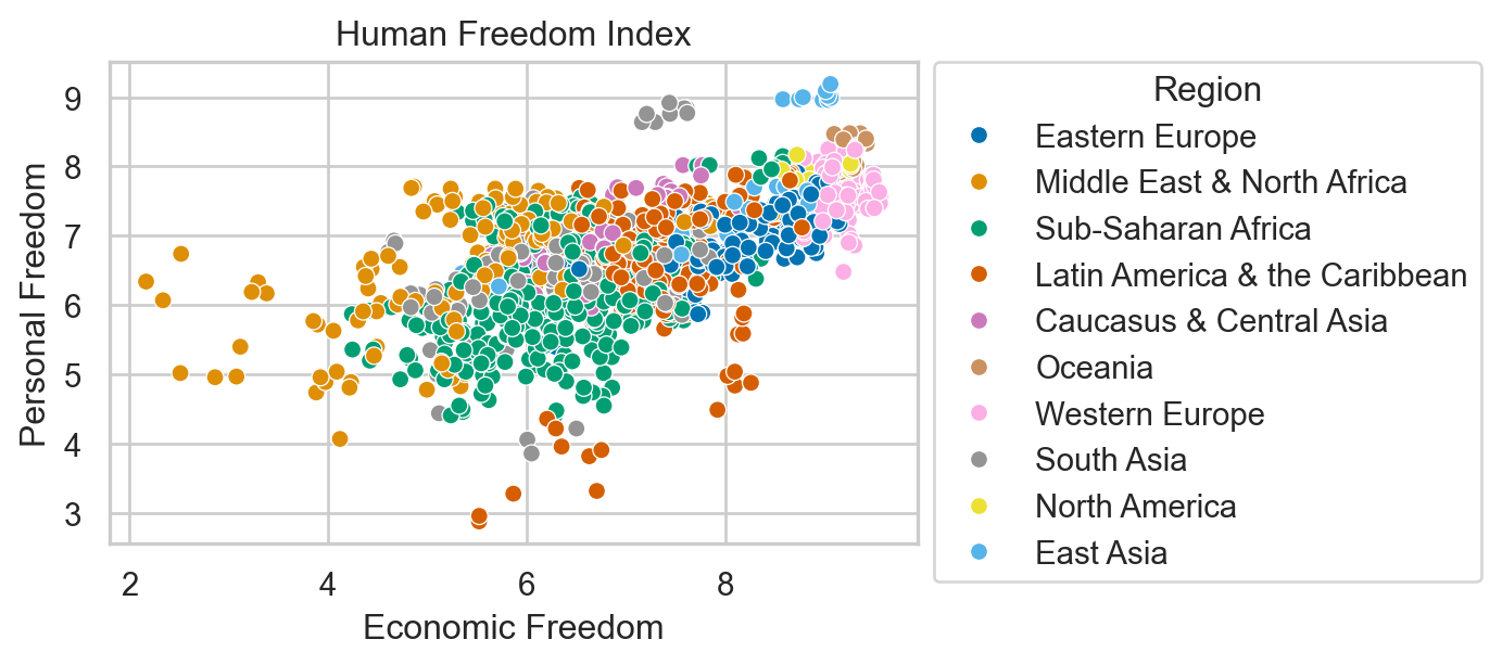
Our data: Human Freedom Index
| year | ISO_code | countries | region | pf_rol_procedural | pf_rol_civil | pf_rol_criminal | pf_rol | pf_ss_homicide | pf_ss_disappearances_disap | ... | ef_regulation_business_bribes | ef_regulation_business_licensing | ef_regulation_business_compliance | ef_regulation_business | ef_regulation | ef_score | ef_rank | hf_score | hf_rank | hf_quartile | |
|---|---|---|---|---|---|---|---|---|---|---|---|---|---|---|---|---|---|---|---|---|---|
| 0 | 2016 | ALB | Albania | Eastern Europe | 6.661503 | 4.547244 | 4.666508 | 5.291752 | 8.920429 | 10.0 | ... | 4.050196 | 7.324582 | 7.074366 | 6.705863 | 6.906901 | 7.54 | 34.0 | 7.568140 | 48.0 | 2.0 |
| 1 | 2016 | DZA | Algeria | Middle East & North Africa | NaN | NaN | NaN | 3.819566 | 9.456254 | 10.0 | ... | 3.765515 | 8.523503 | 7.029528 | 5.676956 | 5.268992 | 4.99 | 159.0 | 5.135886 | 155.0 | 4.0 |
| 2 | 2016 | AGO | Angola | Sub-Saharan Africa | NaN | NaN | NaN | 3.451814 | 8.060260 | 5.0 | ... | 1.945540 | 8.096776 | 6.782923 | 4.930271 | 5.518500 | 5.17 | 155.0 | 5.640662 | 142.0 | 4.0 |
| 3 | 2016 | ARG | Argentina | Latin America & the Caribbean | 7.098483 | 5.791960 | 4.343930 | 5.744791 | 7.622974 | 10.0 | ... | 3.260044 | 5.253411 | 6.508295 | 5.535831 | 5.369019 | 4.84 | 160.0 | 6.469848 | 107.0 | 3.0 |
| 4 | 2016 | ARM | Armenia | Caucasus & Central Asia | NaN | NaN | NaN | 5.003205 | 8.808750 | 10.0 | ... | 4.575152 | 9.319612 | 6.491481 | 6.797530 | 7.378069 | 7.57 | 29.0 | 7.241402 | 57.0 | 2.0 |
5 rows × 123 columns
Understand the data
<class 'pandas.core.frame.DataFrame'>
RangeIndex: 1458 entries, 0 to 1457
Data columns (total 123 columns):
 #    Column                              Dtype
---   ------                              -----
 0    year                                int64
 1    ISO_code                            object
 2    countries                           object
 3    region                              object
 4    pf_rol_procedural                   float64
 5    pf_rol_civil                        float64
 6    pf_rol_criminal                     float64
 7    pf_rol                              float64
 8    pf_ss_homicide                      float64
 9    pf_ss_disappearances_disap          float64
 10   pf_ss_disappearances_violent        float64
 11   pf_ss_disappearances_organized      float64
 12   pf_ss_disappearances_fatalities     float64
 13   pf_ss_disappearances_injuries       float64
 14   pf_ss_disappearances                float64
 15   pf_ss_women_fgm                     float64
 16   pf_ss_women_missing                 float64
 17   pf_ss_women_inheritance_widows      float64
 18   pf_ss_women_inheritance_daughters   float64
 19   pf_ss_women_inheritance             float64
 20   pf_ss_women                         float64
 21   pf_ss                               float64
 22   pf_movement_domestic                float64
 23   pf_movement_foreign                 float64
 24   pf_movement_women                   float64
 25   pf_movement                         float64
 26   pf_religion_estop_establish         float64
 27   pf_religion_estop_operate           float64
 28   pf_religion_estop                   float64
 29   pf_religion_harassment              float64
 30   pf_religion_restrictions            float64
 31   pf_religion                         float64
 32   pf_association_association          float64
 33   pf_association_assembly             float64
 34   pf_association_political_establish  float64
 35   pf_association_political_operate    float64
 36   pf_association_political            float64
 37   pf_association_prof_establish       float64
 38   pf_association_prof_operate         float64
 39   pf_association_prof                 float64
 40   pf_association_sport_establish      float64
 41   pf_association_sport_operate        float64
 42   pf_association_sport                float64
 43   pf_association                      float64
 44   pf_expression_killed                float64
 45   pf_expression_jailed                float64
 46   pf_expression_influence             float64
 47   pf_expression_control               float64
 48   pf_expression_cable                 float64
 49   pf_expression_newspapers            float64
 50   pf_expression_internet              float64
 51   pf_expression                       float64
 52   pf_identity_legal                   float64
 53   pf_identity_parental_marriage       float64
 54   pf_identity_parental_divorce        float64
 55   pf_identity_parental                float64
 56   pf_identity_sex_male                float64
 57   pf_identity_sex_female              float64
 58   pf_identity_sex                     float64
 59   pf_identity_divorce                 float64
 60   pf_identity                         float64
 61   pf_score                            float64
 62   pf_rank                             float64
 63   ef_government_consumption           float64
 64   ef_government_transfers             float64
 65   ef_government_enterprises           float64
 66   ef_government_tax_income            float64
 67   ef_government_tax_payroll           float64
 68   ef_government_tax                   float64
 69   ef_government                       float64
 70   ef_legal_judicial                   float64
 71   ef_legal_courts                     float64
 72   ef_legal_protection                 float64
 73   ef_legal_military                   float64
 74   ef_legal_integrity                  float64
 75   ef_legal_enforcement                float64
 76   ef_legal_restrictions               float64
 77   ef_legal_police                     float64
 78   ef_legal_crime                      float64
 79   ef_legal_gender                     float64
 80   ef_legal                            float64
 81   ef_money_growth                     float64
 82   ef_money_sd                         float64
 83   ef_money_inflation                  float64
 84   ef_money_currency                   float64
 85   ef_money                            float64
 86   ef_trade_tariffs_revenue            float64
 87   ef_trade_tariffs_mean               float64
 88   ef_trade_tariffs_sd                 float64
 89   ef_trade_tariffs                    float64
 90   ef_trade_regulatory_nontariff       float64
 91   ef_trade_regulatory_compliance      float64
 92   ef_trade_regulatory                 float64
 93   ef_trade_black                      float64
 94   ef_trade_movement_foreign           float64
 95   ef_trade_movement_capital           float64
 96   ef_trade_movement_visit             float64
 97   ef_trade_movement                   float64
 98   ef_trade                            float64
 99   ef_regulation_credit_ownership      float64
 100  ef_regulation_credit_private        float64
 101  ef_regulation_credit_interest       float64
 102  ef_regulation_credit                float64
 103  ef_regulation_labor_minwage         float64
 104  ef_regulation_labor_firing          float64
 105  ef_regulation_labor_bargain         float64
 106  ef_regulation_labor_hours           float64
 107  ef_regulation_labor_dismissal       float64
 108  ef_regulation_labor_conscription    float64
 109  ef_regulation_labor                 float64
 110  ef_regulation_business_adm          float64
 111  ef_regulation_business_bureaucracy  float64
 112  ef_regulation_business_start        float64
 113  ef_regulation_business_bribes       float64
 114  ef_regulation_business_licensing    float64
 115  ef_regulation_business_compliance   float64
 116  ef_regulation_business              float64
 117  ef_regulation                       float64
 118  ef_score                            float64
 119  ef_rank                             float64
 120  hf_score                            float64
 121  hf_rank                             float64
 122  hf_quartile                         float64
dtypes: float64(119), int64(1), object(3)
memory usage: 1.4+ MB| year | pf_rol_procedural | pf_rol_civil | pf_rol_criminal | pf_rol | pf_ss_homicide | pf_ss_disappearances_disap | pf_ss_disappearances_violent | pf_ss_disappearances_organized | pf_ss_disappearances_fatalities | ... | ef_regulation_business_bribes | ef_regulation_business_licensing | ef_regulation_business_compliance | ef_regulation_business | ef_regulation | ef_score | ef_rank | hf_score | hf_rank | hf_quartile | |
|---|---|---|---|---|---|---|---|---|---|---|---|---|---|---|---|---|---|---|---|---|---|
| count | 1458.000000 | 880.000000 | 880.000000 | 880.000000 | 1378.000000 | 1378.000000 | 1369.000000 | 1378.000000 | 1279.000000 | 1378.000000 | ... | 1283.000000 | 1357.000000 | 1368.000000 | 1374.000000 | 1378.000000 | 1378.000000 | 1378.000000 | 1378.000000 | 1378.000000 | 1378.000000 |
| mean | 2012.000000 | 5.589355 | 5.474770 | 5.044070 | 5.309641 | 7.412980 | 8.341855 | 9.519458 | 6.772869 | 9.584972 | ... | 4.886192 | 7.698494 | 6.981858 | 6.317668 | 7.019782 | 6.785610 | 76.973149 | 6.993444 | 77.007983 | 2.490566 |
| std | 2.582875 | 2.080957 | 1.428494 | 1.724886 | 1.529310 | 2.832947 | 3.225902 | 1.744673 | 2.768983 | 1.559826 | ... | 1.889168 | 1.728507 | 1.979200 | 1.230988 | 1.027625 | 0.883601 | 44.540142 | 1.025811 | 44.506549 | 1.119698 |
| min | 2008.000000 | 0.000000 | 0.000000 | 0.000000 | 0.000000 | 0.000000 | 0.000000 | 0.000000 | 0.000000 | 0.000000 | ... | 0.000000 | 0.000000 | 0.000000 | 2.009841 | 2.483540 | 2.880000 | 1.000000 | 3.765827 | 1.000000 | 1.000000 |
| 25% | 2010.000000 | 4.133333 | 4.549550 | 3.789724 | 4.131746 | 6.386978 | 10.000000 | 10.000000 | 5.000000 | 9.942607 | ... | 3.433786 | 6.874687 | 6.368178 | 5.591851 | 6.429498 | 6.250000 | 38.000000 | 6.336685 | 39.000000 | 1.000000 |
| 50% | 2012.000000 | 5.300000 | 5.300000 | 4.575189 | 4.910797 | 8.638278 | 10.000000 | 10.000000 | 7.500000 | 10.000000 | ... | 4.418371 | 8.074161 | 7.466692 | 6.265234 | 7.082075 | 6.900000 | 77.000000 | 6.923840 | 76.000000 | 2.000000 |
| 75% | 2014.000000 | 7.389499 | 6.410975 | 6.400000 | 6.513178 | 9.454402 | 10.000000 | 10.000000 | 10.000000 | 10.000000 | ... | 6.227978 | 8.991882 | 8.209310 | 7.139718 | 7.720955 | 7.410000 | 115.000000 | 7.894660 | 115.000000 | 3.000000 |
| max | 2016.000000 | 9.700000 | 8.773533 | 8.719848 | 8.723094 | 9.926568 | 10.000000 | 10.000000 | 10.000000 | 10.000000 | ... | 9.623811 | 9.999638 | 9.865488 | 9.272600 | 9.439828 | 9.190000 | 162.000000 | 9.126313 | 162.000000 | 4.000000 |
8 rows × 120 columns
Identifying missing values
year                   0
ISO_code               0
countries              0
region                 0
pf_rol_procedural    578
                    ...
ef_score              80
ef_rank               80
hf_score              80
hf_rank               80
hf_quartile           80
Length: 123, dtype: int64
A lot of missing values 🙃
Data Cleaning
Handling missing data
Options
- Do nothing…
- Remove them
- Imputate
We will be using pf_score from hsi: 80 missing values
Imputation
In statistics, imputation is the process of replacing missing data with substituted values.
Considerations
- Data distribution
- Impact on analysis
- Missing data mechanism
- Multiple imputation
- Can also be used on outliers
Mean imputation
How it Works: Replace missing values with the arithmetic mean of the non-missing values in the same variable.
Pros:
- Easy and fast.
- Works well with small numerical datasets
Cons:
- It only works on the column level.
- Will give poor results on encoded categorical features.
- Not very accurate.
- Doesn’t account for the uncertainty in the imputations.
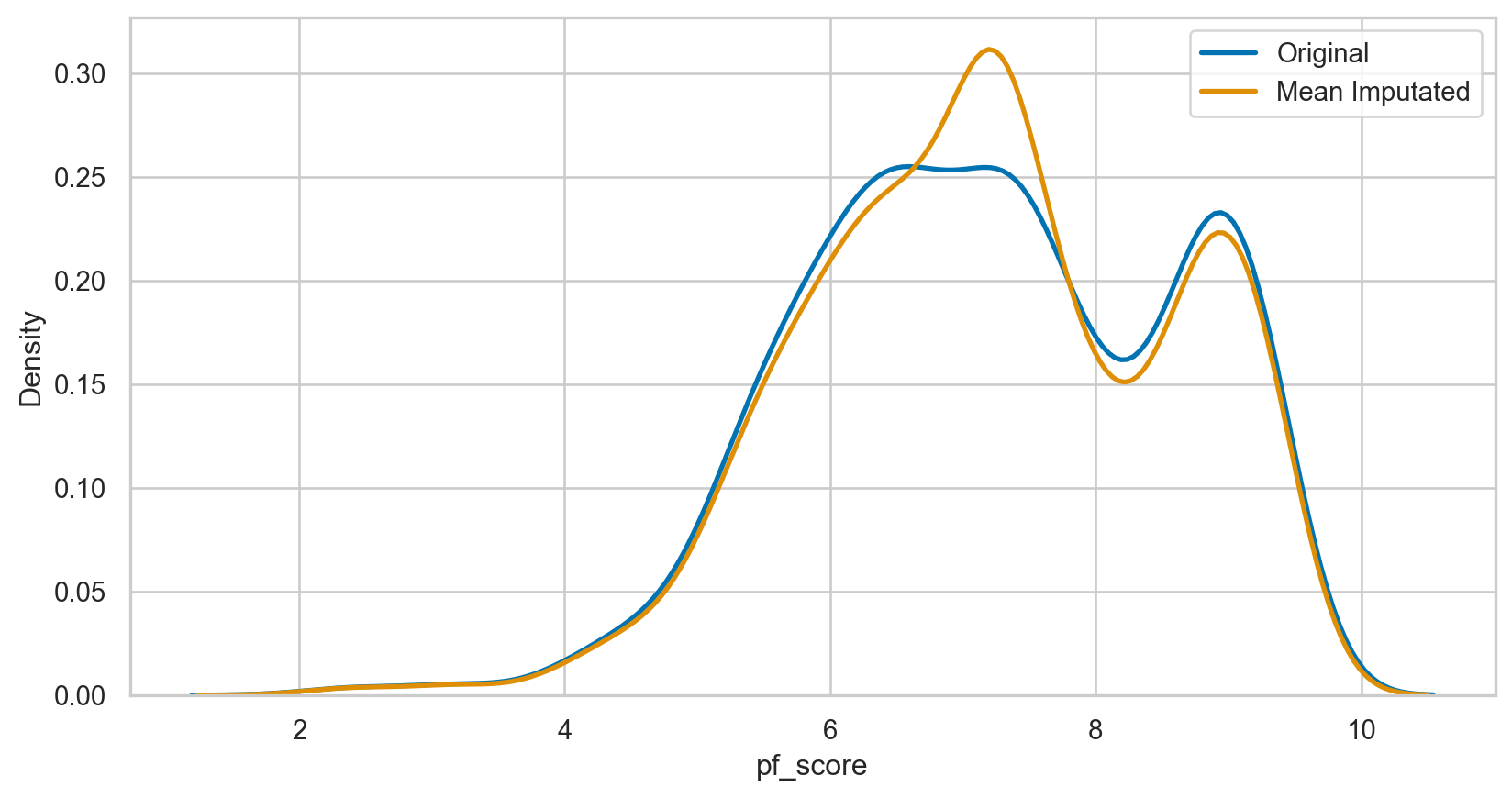
hfi_copy = hfi

mean_imputer = SimpleImputer(strategy = 'mean')
hfi_copy['mean_pf_score'] = mean_imputer.fit_transform(hfi_copy[['pf_score']])

mean_plot = sns.kdeplot(data = hfi_copy, x = 'pf_score', linewidth = 2, label = "Original")

mean_plot = sns.kdeplot(data = hfi_copy, x = 'mean_pf_score', linewidth = 2, label = "Mean Imputated")

plt.legend()

plt.show()
Median imputation
How it Works: Replace missing values with the median of the non-missing values in the same variable.
Pros (same as mean):
- Easy and fast.
- Works well with small numerical datasets
Cons (same as mean):
- It only works on the column level.
- Will give poor results on encoded categorical features.
- Not very accurate.
- Doesn’t account for the uncertainty in the imputations.
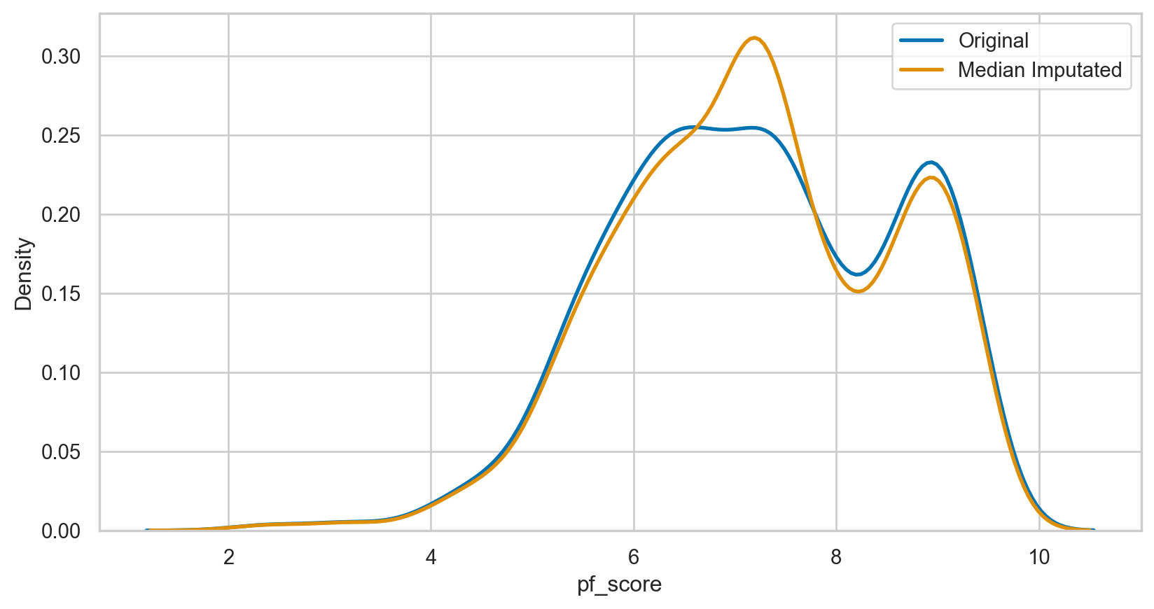
median_imputer = SimpleImputer(strategy = 'median')
hfi_copy['median_pf_score'] = median_imputer.fit_transform(hfi_copy[['pf_score']])

median_plot = sns.kdeplot(data = hfi_copy, x = 'pf_score', linewidth = 2, label = "Original")

median_plot = sns.kdeplot(data = hfi_copy, x = 'median_pf_score', linewidth = 2, label = "Median Imputated")

plt.legend()

plt.show()
Data type conversion
| year | ISO_code | countries | region | pf_rol_procedural | pf_rol_civil | pf_rol_criminal | pf_rol | pf_ss_homicide | pf_ss_disappearances_disap | ... | ef_regulation_business_compliance | ef_regulation_business | ef_regulation | ef_score | ef_rank | hf_score | hf_rank | hf_quartile | mean_pf_score | median_pf_score | |
|---|---|---|---|---|---|---|---|---|---|---|---|---|---|---|---|---|---|---|---|---|---|
| 0 | 2016-01-01 | ALB | Albania | Eastern Europe | 6.661503 | 4.547244 | 4.666508 | 5.291752 | 8.920429 | 10.0 | ... | 7.074366 | 6.705863 | 6.906901 | 7.54 | 34.0 | 7.56814 | 48.0 | 2.0 | 7.596281 | 7.596281 |
1 rows × 125 columns
Removing duplicates
<class 'pandas.core.frame.DataFrame'>
RangeIndex: 1458 entries, 0 to 1457
Columns: 125 entries, year to median_pf_score
dtypes: datetime64[ns](1), float64(121), object(3)
memory usage: 1.4+ MB<class 'pandas.core.frame.DataFrame'>
RangeIndex: 1458 entries, 0 to 1457
Columns: 125 entries, year to median_pf_score
dtypes: datetime64[ns](1), float64(121), object(3)
memory usage: 1.4+ MBNo duplicates! 😊
Dimensional reduction
Dimension reduction, is the transformation of data from a high-dimensional space into a low-dimensional space so that the low-dimensional representation retains some meaningful properties of the original data, ideally close to its intrinsic dimension.
Principal component analysis (PCA) - Unsupervised
Maximizes variance in the dataset.
Finds orthogonal principal components.
Useful for feature extraction and data visualization.
Dimensional reduction: applied
numeric_cols = hfi.select_dtypes(include = [np.number]).columns

# Applying mean imputation only to numeric columns
hfi[numeric_cols] = hfi[numeric_cols].fillna(hfi[numeric_cols].mean())

features = ['pf_rol_procedural', 'pf_rol_civil', 'pf_rol_criminal', 'pf_rol', 'hf_score', 'hf_rank', 'hf_quartile']

x = hfi.loc[:, features].values
y = hfi.loc[:, 'region'].values
x = StandardScaler().fit_transform(x)
Code
pca = PCA(n_components = 2)
principalComponents = pca.fit_transform(x)
principalDf = pd.DataFrame(data = principalComponents, columns = ['principal component 1', 'principal component 2'])
pca_variance_explained = pca.explained_variance_ratio_
print("Variance explained:", pca_variance_explained, "\n", principalDf)
Variance explained: [0.76138995 0.15849799]
principal component 1 principal component 2
0 5.164625e-01 -9.665680e-01
1 -2.366765e+00 1.957381e+00
2 -2.147729e+00 1.664483e+00
3 -2.784437e-01 8.066415e-01
4 3.716205e-01 -4.294282e-01
... ... ...
1453 -4.181375e+00 -4.496988e-01
1454 -5.213024e-01 6.010449e-01
1455 1.374342e-16 -2.907121e-16
1456 -1.545577e+00 -5.422255e-01
1457 -3.669011e+00 4.294948e-01
[1458 rows x 2 columns]Code
# Combining the scatterplot of principal components with the scree plot using the correct column names
fig, axes = plt.subplots(nrows = 1, ncols = 2, figsize = (12, 5))

# Scatterplot of Principal Components
axes[0].scatter(principalDf['principal component 1'], principalDf['principal component 2'])
for i in range(len(pca.components_)):
    axes[0].arrow(0, 0, pca.components_[i, 0], pca.components_[i, 1], head_width = 0.1, head_length = 0.15, fc = 'r', ec = 'r', linewidth = 2)
    axes[0].text(pca.components_[i, 0] * 1.2, pca.components_[i, 1] * 1.2, f'Eigenvector {i+1}', color = 'r', fontsize = 12)
axes[0].set_xlabel('Principal Component 1')
axes[0].set_ylabel('Principal Component 2')
axes[0].set_title('Scatterplot of Principal Components with Eigenvectors')
axes[0].grid()

# Scree Plot for PCA
axes[1].bar(range(1, len(pca_variance_explained) + 1), pca_variance_explained, alpha = 0.6, color = 'g', label = 'Individual Explained Variance')
axes[1].set_ylabel('Explained variance ratio')
axes[1].set_xlabel('Principal components')
axes[1].set_title('Scree Plot for PCA')
axes[1].legend(loc='best')

plt.tight_layout()
plt.show()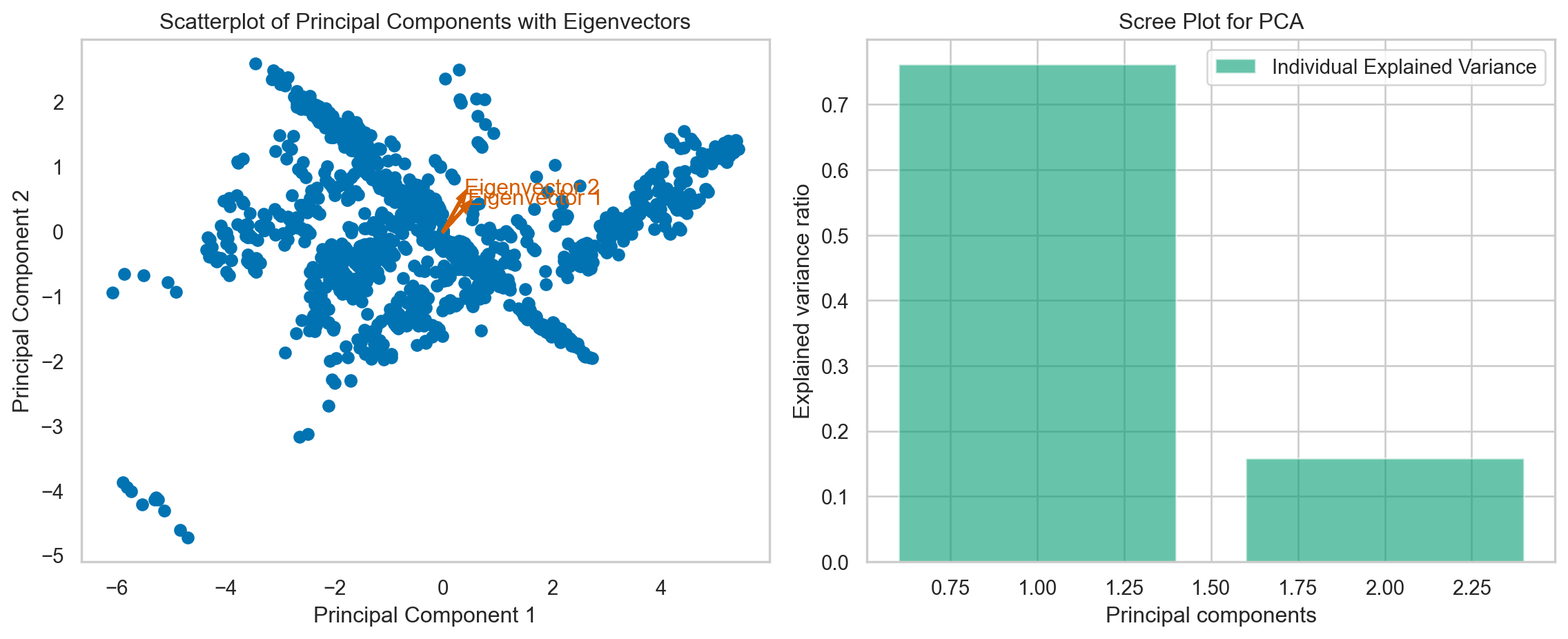
So, that’s it?
…Not really
Find the optimal number of components.
Code
# Assuming hfi DataFrame is already defined and loaded

# Select numerical columns
numerical_cols = hfi.select_dtypes(include=['int64', 'float64']).columns

# Scale the data
scaler = StandardScaler()
scaled_data = scaler.fit_transform(hfi[numerical_cols])

# Apply PCA
pca = PCA().fit(scaled_data)

# Get explained variance ratio and cumulative explained variance
explained_variance_ratio = pca.explained_variance_ratio_
cumulative_explained_variance = explained_variance_ratio.cumsum()

# Decide number of components to retain 75% variance
threshold = 0.75
num_components = next(i for i, cumulative_var in enumerate(cumulative_explained_variance) if cumulative_var >= threshold) + 1

# Plot the explained variance
plt.figure(figsize=(10, 6))
plt.plot(range(1, len(cumulative_explained_variance) + 1), cumulative_explained_variance, marker='o', linestyle='--')
plt.axhline(y=threshold, color='r', linestyle='-')
plt.axvline(x=num_components, color='r', linestyle='-')
plt.annotate(f'{num_components} components', xy=(num_components, threshold), xytext=(num_components+5, threshold-0.05),
             arrowprops=dict(color='r', arrowstyle='->'),
             fontsize=12, color='r')
plt.title('Cumulative Explained Variance by Principal Components')
plt.xlabel('Principal Component')
plt.ylabel('Cumulative Explained Variance')
plt.grid(True)
plt.show()

print(f"Number of components to retain 75% variance: {num_components}")

# Apply PCA with the chosen number of components
pca = PCA(n_components=num_components)
reduced_data = pca.fit_transform(scaled_data)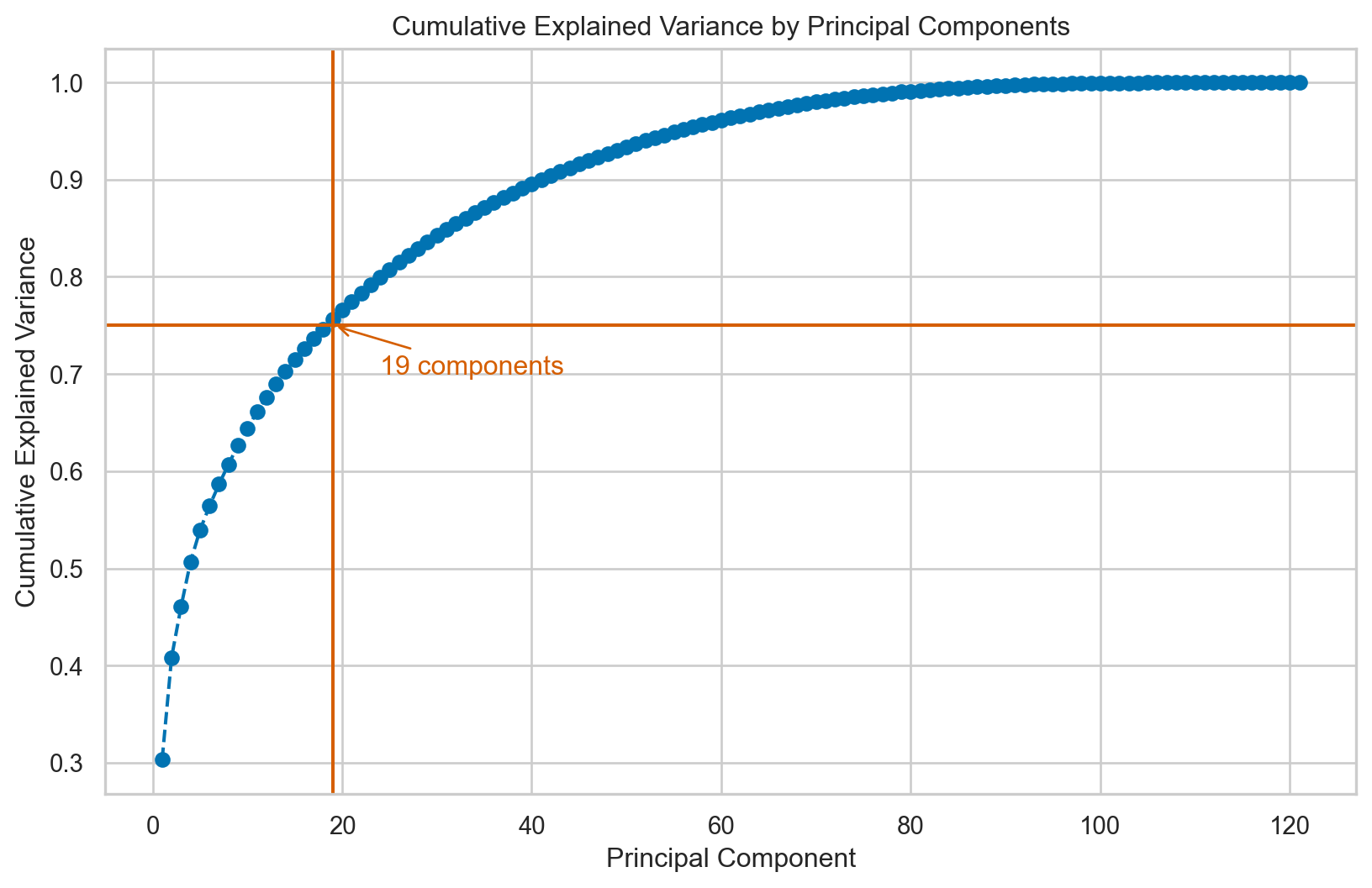
Number of components to retain 75% variance: 19Dimensional reduction: what now?
Feature Selection: Choose the most informative components.
Visualization: Graph the reduced dimensions to identify patterns.
Clustering: Group similar data points using clustering algorithms.
Classification: Predict categories using classifiers on reduced features.
Model Evaluation: Assess model performance with metrics like accuracy.
Cross-Validation: Validate model stability with cross-validation.
Hyperparameter Tuning: Optimize model settings for better performance.
Model Interpretation: Understand feature influence in the models.
Ensemble Methods: Improve predictions by combining multiple models.
Deployment: Deploy the model for real-world predictions.
Iterative Refinement: Refine analysis based on initial results.
Reporting: Summarize findings for stakeholders.
Clustering
Setup
# Data Handling and Manipulation
import pandas as pd
import numpy as np

# Data Preprocessing
from sklearn.preprocessing import StandardScaler, OneHotEncoder
from sklearn.compose import ColumnTransformer
from sklearn.pipeline import Pipeline
from sklearn.impute import SimpleImputer
from sklearn.decomposition import PCA

# Model Selection and Evaluation
from sklearn.model_selection import train_test_split, GridSearchCV, RandomizedSearchCV
from sklearn.metrics import silhouette_score, davies_bouldin_score, calinski_harabasz_score
from sklearn.mixture import GaussianMixture

# Clustering Models
from sklearn.cluster import KMeans

# Data Visualization
import matplotlib.pyplot as plt
import seaborn as sns

# Set the default style for visualization
sns.set_theme(style = "white", palette = "colorblind")

# Increase font size of all Seaborn plot elements
sns.set(font_scale = 1.25)
Unsupervised Learning
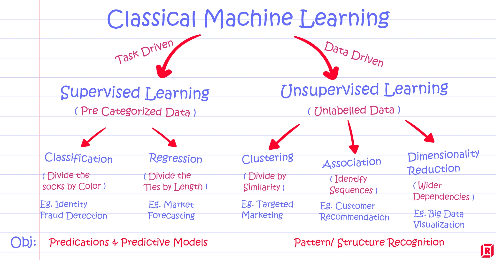
Clustering
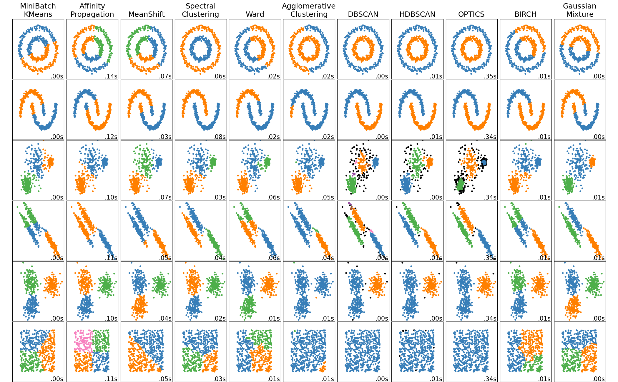
Clustering
Some use cases for clustering include:
-
- Grouping together users with similar viewing patterns on Netflix, in order to recommend similar content
-
- Fraud detection, detecting defective mechanical parts
Genetics:
- Clustering DNA patterns to analyze evolutionary biology
Customer segmentation:
- Understanding different customer segments to devise marketing strategies
Question
How well can we cluster freedom index scores?
Our data: PCA reduced Human Freedom Index
data = pd.DataFrame(reduced_data)
data.rename(columns=lambda x: f'pc_{x}', inplace=True)
data.head()| pc_0 | pc_1 | pc_2 | pc_3 | pc_4 | pc_5 | pc_6 | pc_7 | pc_8 | pc_9 | pc_10 | pc_11 | pc_12 | pc_13 | pc_14 | pc_15 | pc_16 | pc_17 | pc_18 | |
|---|---|---|---|---|---|---|---|---|---|---|---|---|---|---|---|---|---|---|---|
| 0 | 2.779418 | -0.498626 | 0.469355 | 3.387443 | 0.567041 | 1.296449 | -0.454311 | 0.047696 | -0.150022 | -1.206748 | 2.647105 | 0.583670 | -0.213672 | 1.608173 | -0.374059 | -0.490913 | -0.132991 | -0.403151 | -0.991481 |
| 1 | -9.374297 | 0.647491 | -4.321327 | -4.695802 | -0.672385 | 3.209548 | -0.378487 | -3.215965 | -1.908267 | 0.129144 | 0.595631 | 0.347146 | -0.249731 | -2.302677 | -0.102451 | 0.297895 | 1.443028 | -2.022844 | 0.943593 |
| 2 | -8.850868 | -2.931088 | 2.220075 | -2.100491 | -0.818193 | 0.224287 | -1.318509 | 0.308495 | -4.324757 | -1.111543 | 0.689022 | -1.816347 | 1.090664 | -0.404623 | 1.047847 | 0.230615 | 0.151937 | 0.683630 | 3.053161 |
| 3 | -1.708081 | -6.713719 | 2.768734 | -5.725613 | -1.733888 | -1.348572 | -4.638082 | -1.049769 | -3.157522 | 0.848578 | -0.132706 | 3.154590 | -0.318503 | -3.688724 | -1.217743 | -0.400556 | 3.205119 | -0.621442 | -1.703220 |
| 4 | 1.640691 | 2.223795 | 2.299552 | 0.792827 | -2.449994 | 0.373804 | 2.057514 | -1.241613 | 0.767273 | 0.386597 | 0.679367 | -0.893322 | -1.659838 | -0.013696 | 0.463806 | 0.941999 | 0.872254 | 0.104267 | -0.210407 |
Clustering methods
K-Means Clustering
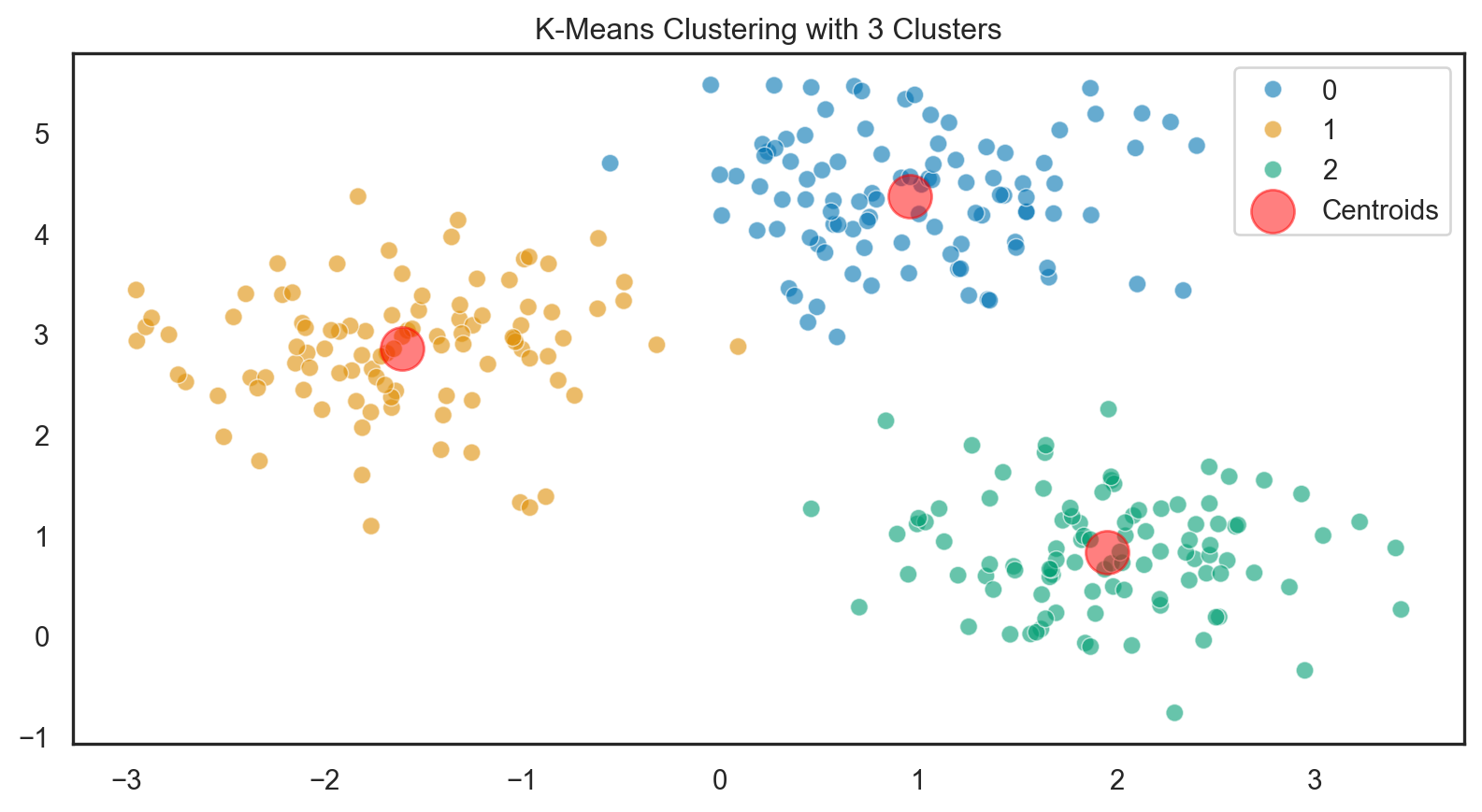
The goal of K-Means is to minimize the variance within each cluster. The variance is measured as the sum of squared distances between each point and its corresponding cluster centroid. The objective function, which K-Means aims to minimize, can be defined as:
\(J = \sum_{i=1}^{k} \sum_{x \in C_i} ||x - \mu_i||^2\)
Where:
\(J\) is the objective function
\(k\) is the number of clusters
\(C_i\) is the set of points belonging to a cluster \(i\).
\(x\) is a point in the cluster \(C_i\)
\(||x - \mu_i||^2\) is the squared Euclidean distance between a point \(x\) and the centroid \(\mu_i\), which measures the dissimilarity between them.
Initialization: Randomly selects \(k\) initial centroids.
Assignment Step: Assigns each data point to the closest centroid based on Euclidean distance.
Update Step: Recalculates centroids as the mean of assigned points in each cluster.
Convergence: Iterates until the centroids stabilize (minimal change from one iteration to the next).
Objective: Minimizes the within-cluster sum of squares (WCSS), the sum of squared distances between points and their corresponding centroid.
Optimal \(k\): Determined experimentally, often using methods like the Elbow Method.
Sensitivity: Results can vary based on initial centroid selection; techniques like “k-means++” improve initial centroid choices.
Efficiency: Generally good, but worsens with increasing \(k\) and data dimensionality; sensitive to outliers.
Choosing the right number of clusters
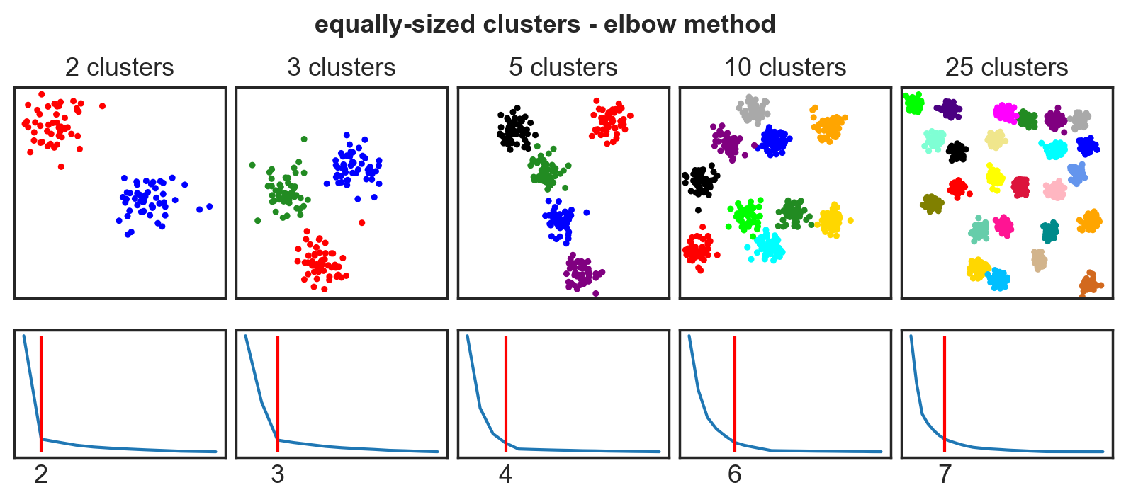
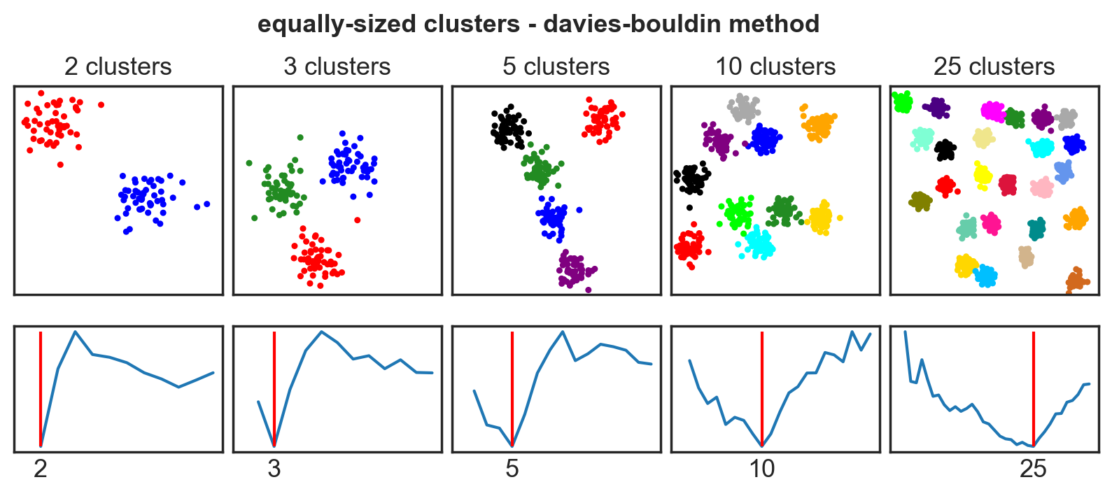
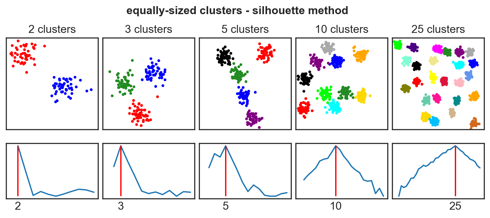
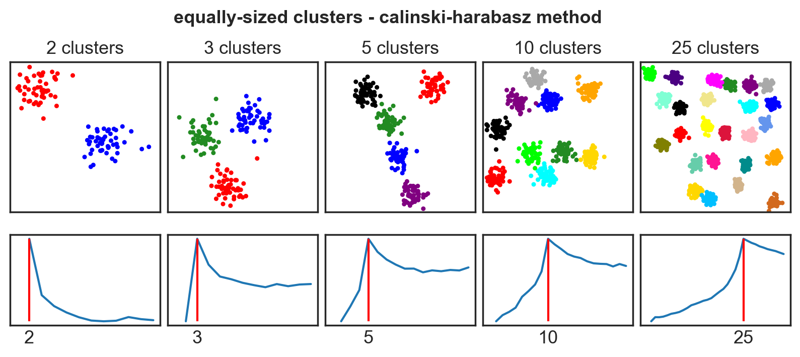
Four main methods:
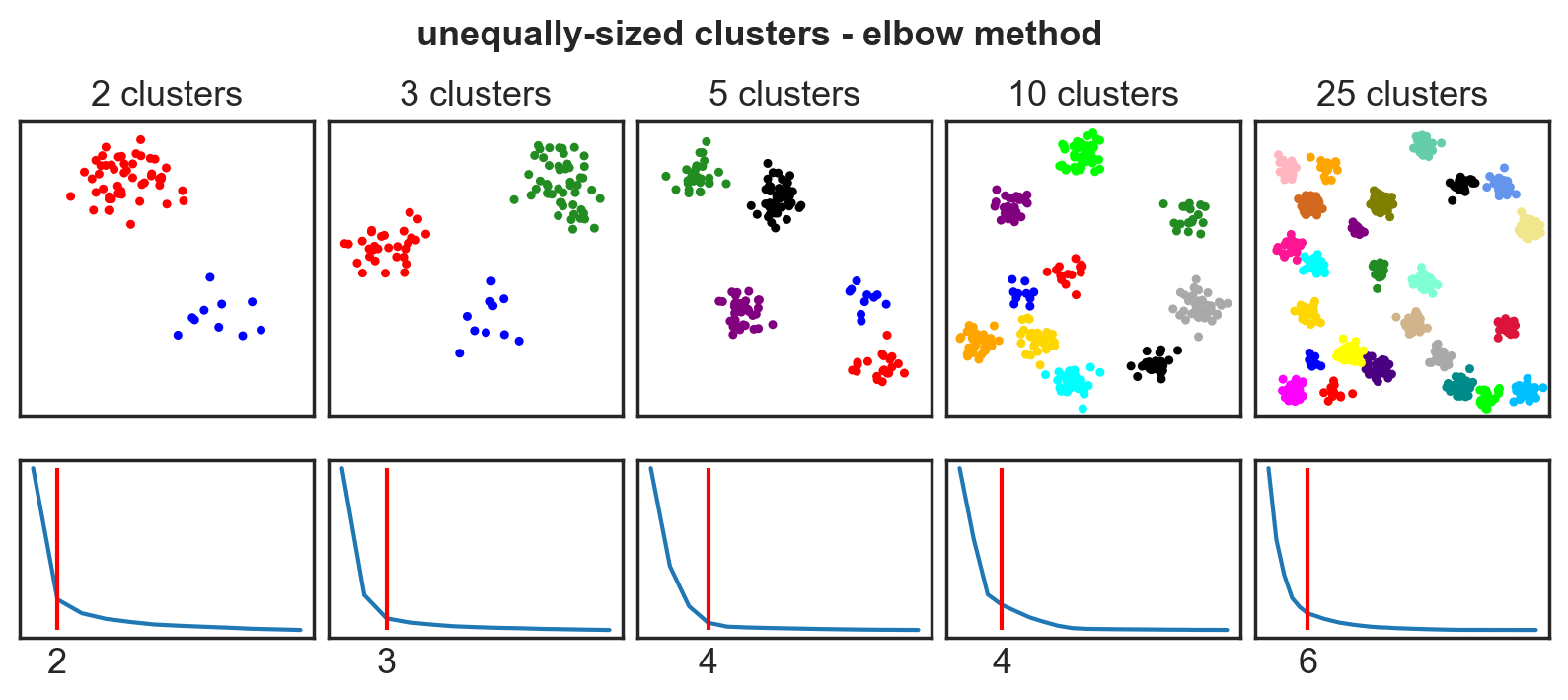
Elbow Method
- Identifies the \(k\) at which the within-cluster sum of squares (WCSS) starts to diminish more slowly.
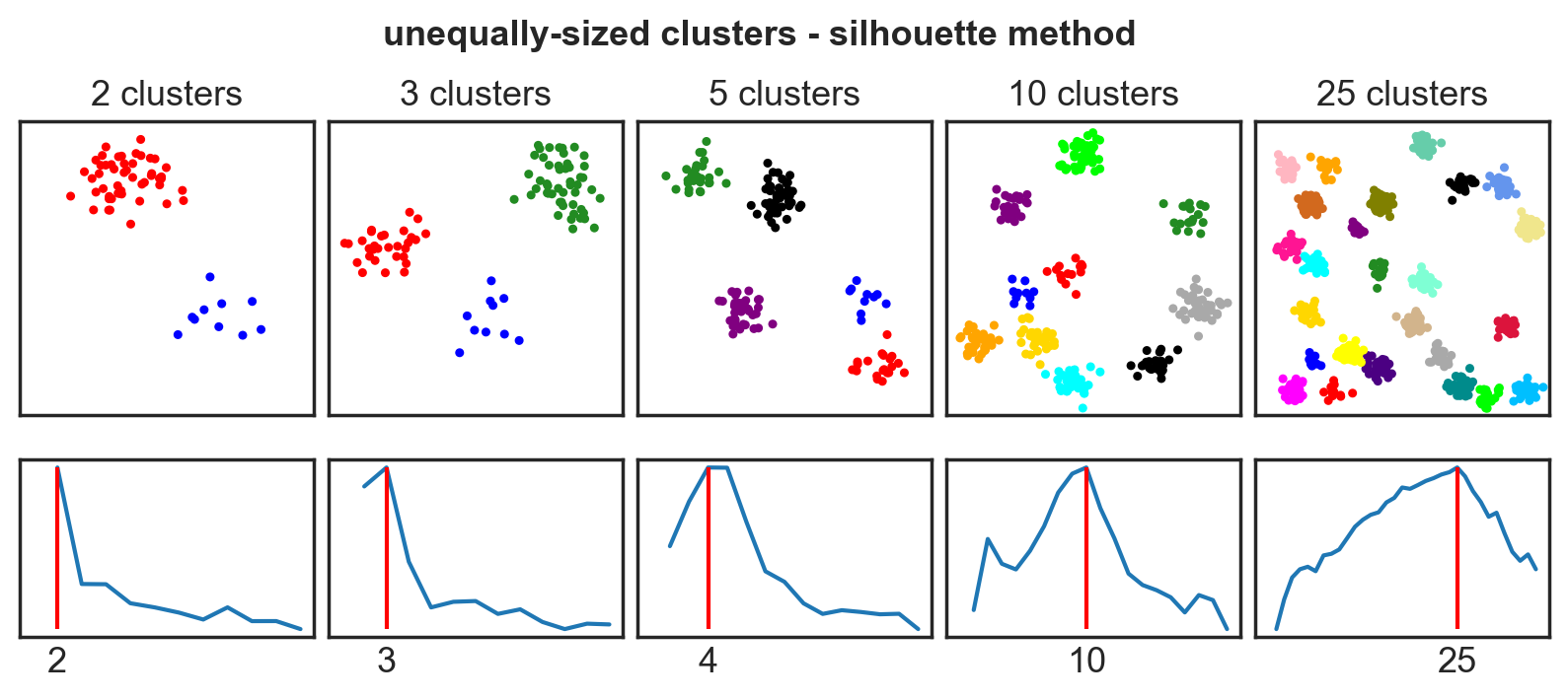
Silhouette Score
- Measures how similar an object is to its own cluster compared to other clusters.
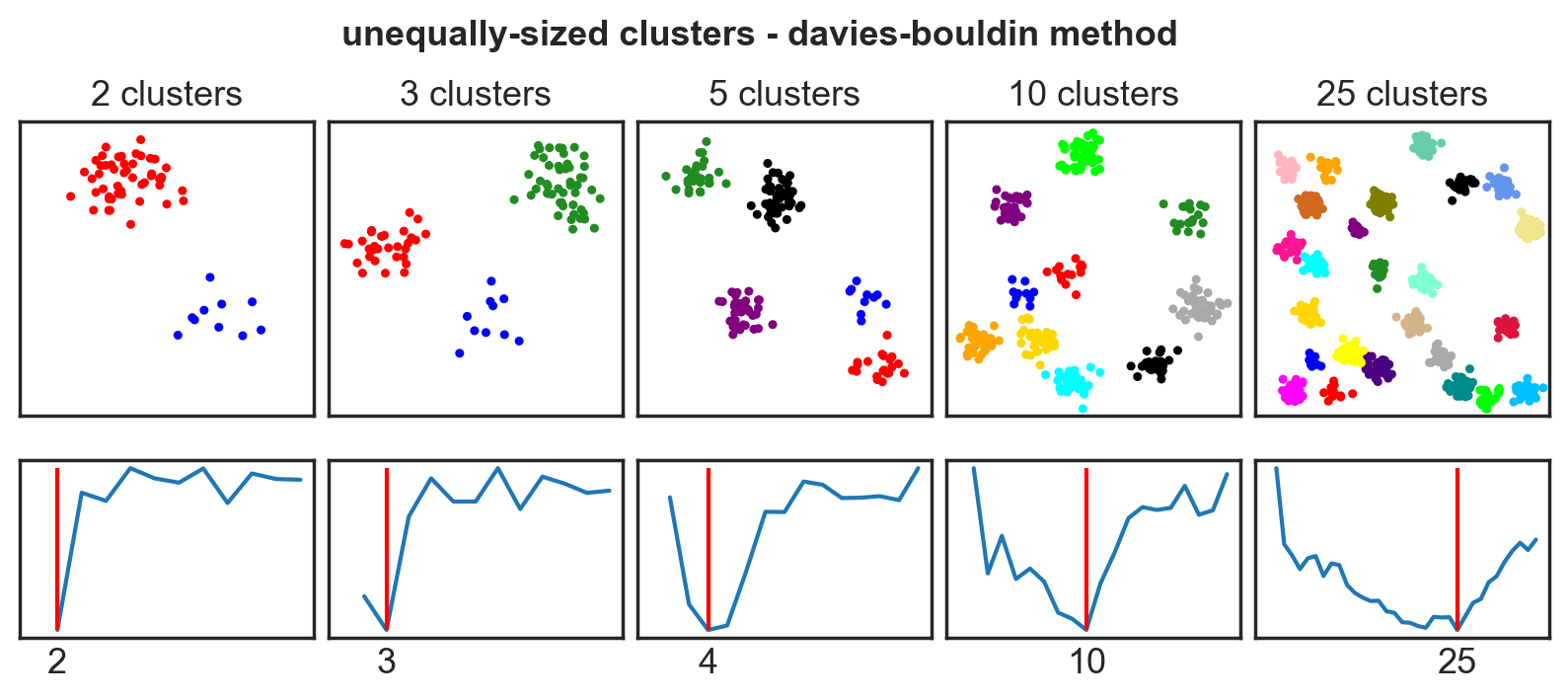
Davies-Bouldin Index
- Evaluates intra-cluster similarity and inter-cluster differences.
Calinski-Harabasz Index (Variance Ratio Criterion)
- Measures the ratio of the sum of between-clusters dispersion and of intra-cluster dispersion for all clusters.
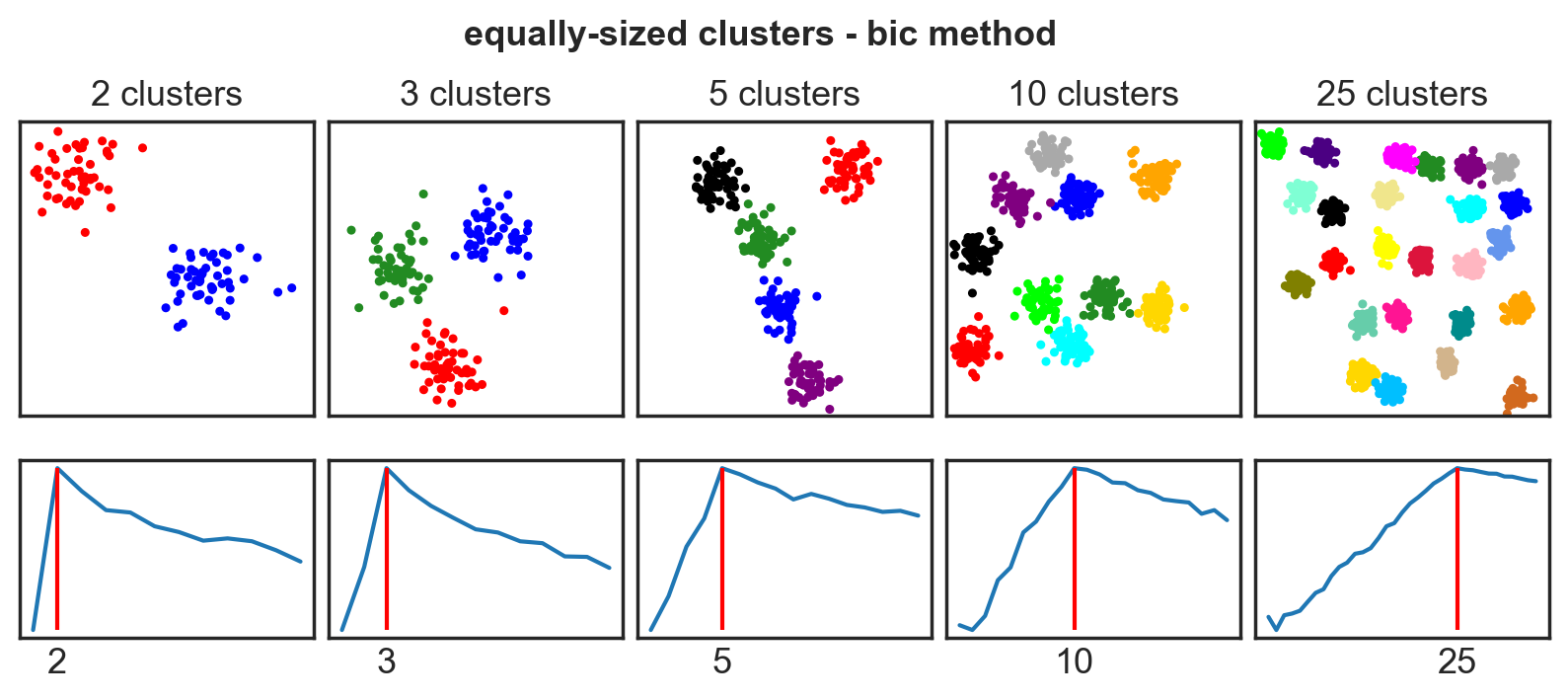
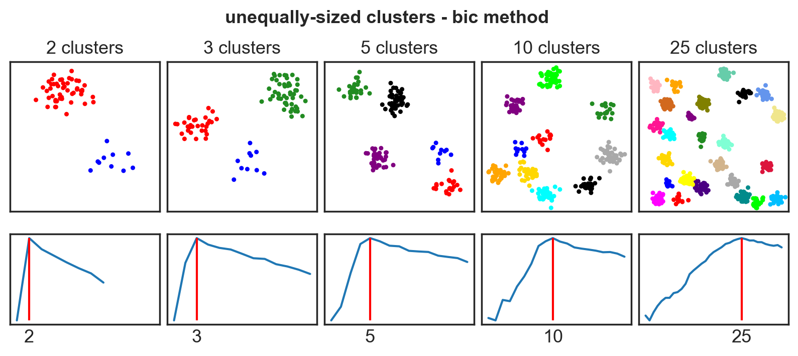
BIC
- Identifies the optimal number of clusters by penalizing models for excessive parameters, striking a balance between simplicity and accuracy.
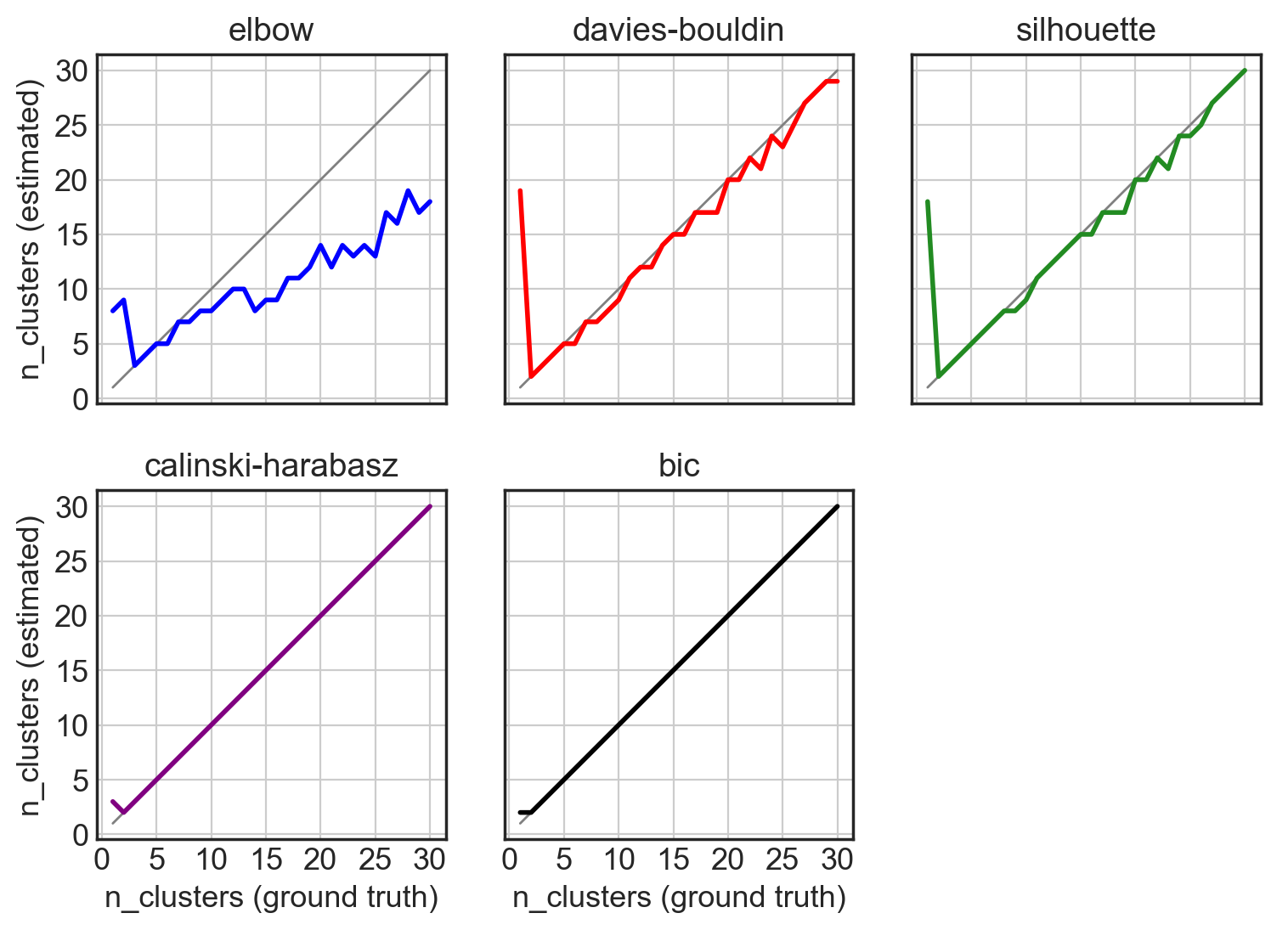
Systematic comparison: Equal clusters
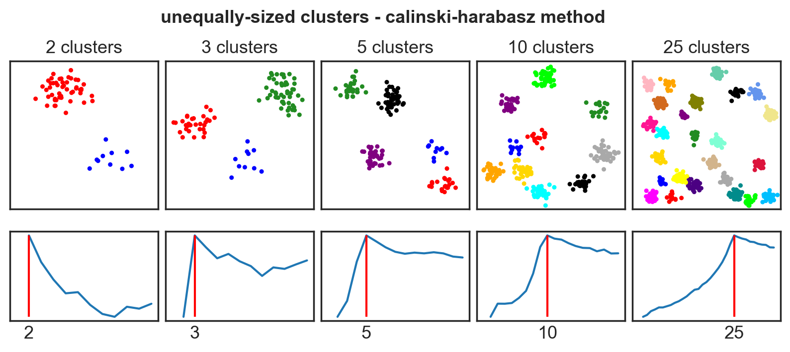
Systematic comparison: Unequal clusters
Systematic comparison - accuracy
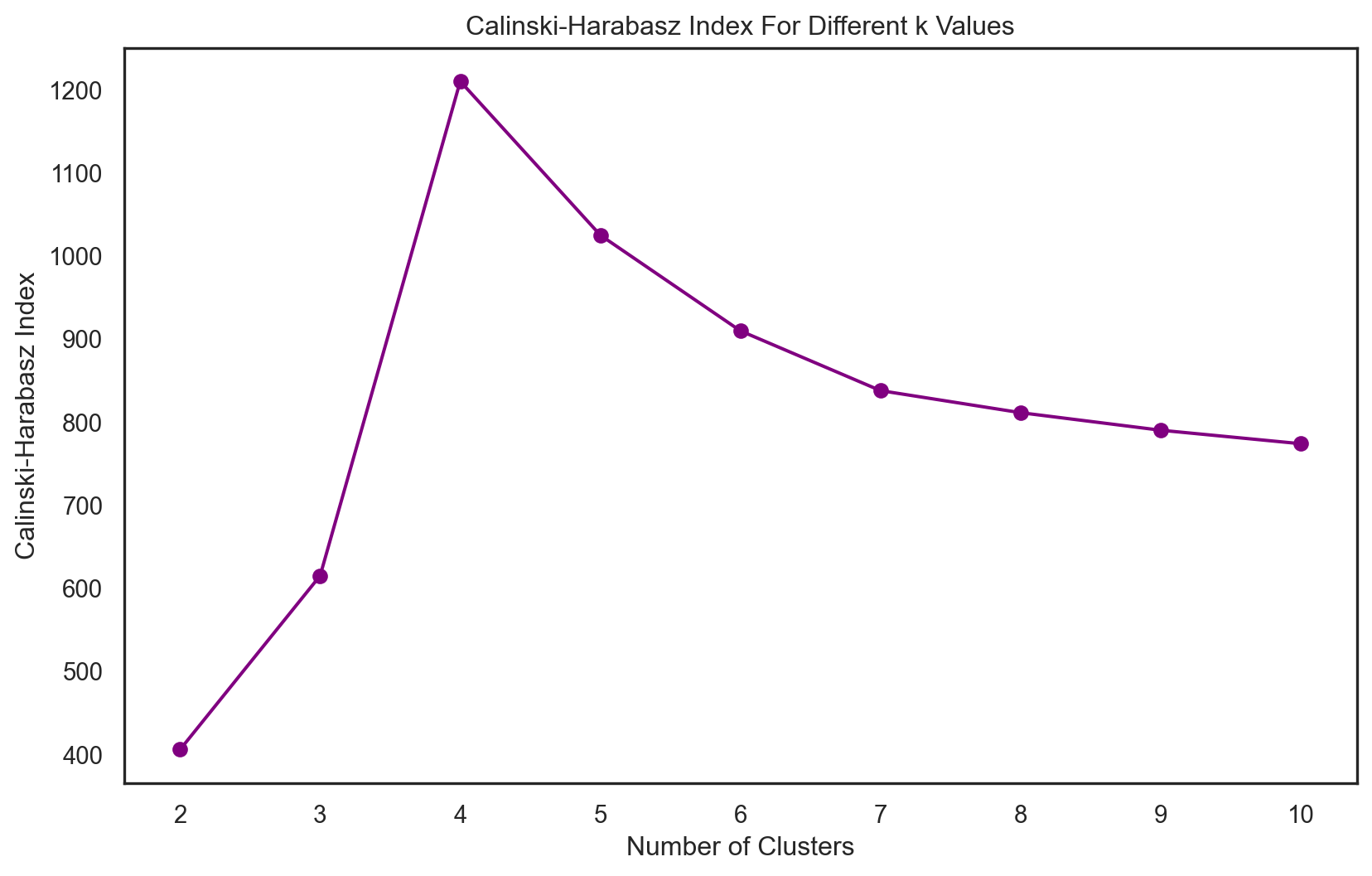
Calinski-Harabasz Index
\(CH = \frac{SS_B / (k - 1)}{SS_W / (n - k)}\)
where:
\(CH\) is the Calinski-Harabasz score.
\(SS_B\) is the between-cluster variance.
\(SS_W\) is the within-cluster variance.
\(k\) is the number of clusters.
\(n\) is the number of data points.
Pros:
Clear Interpretation: High values indicate better-defined clusters.
Computationally Efficient: Less resource-intensive than many alternatives.
Scale-Invariant: Effective across datasets of varying sizes.
No Labeled Data Required: Useful for unsupervised learning scenarios.
Cons:
Cluster Structure Bias: Prefers convex clusters of similar sizes.
Sample Size Sensitivity: Can favor more clusters in larger datasets.
Not Ideal for Overlapping Clusters: Assumes distinct, non-overlapping clusters.
BIC
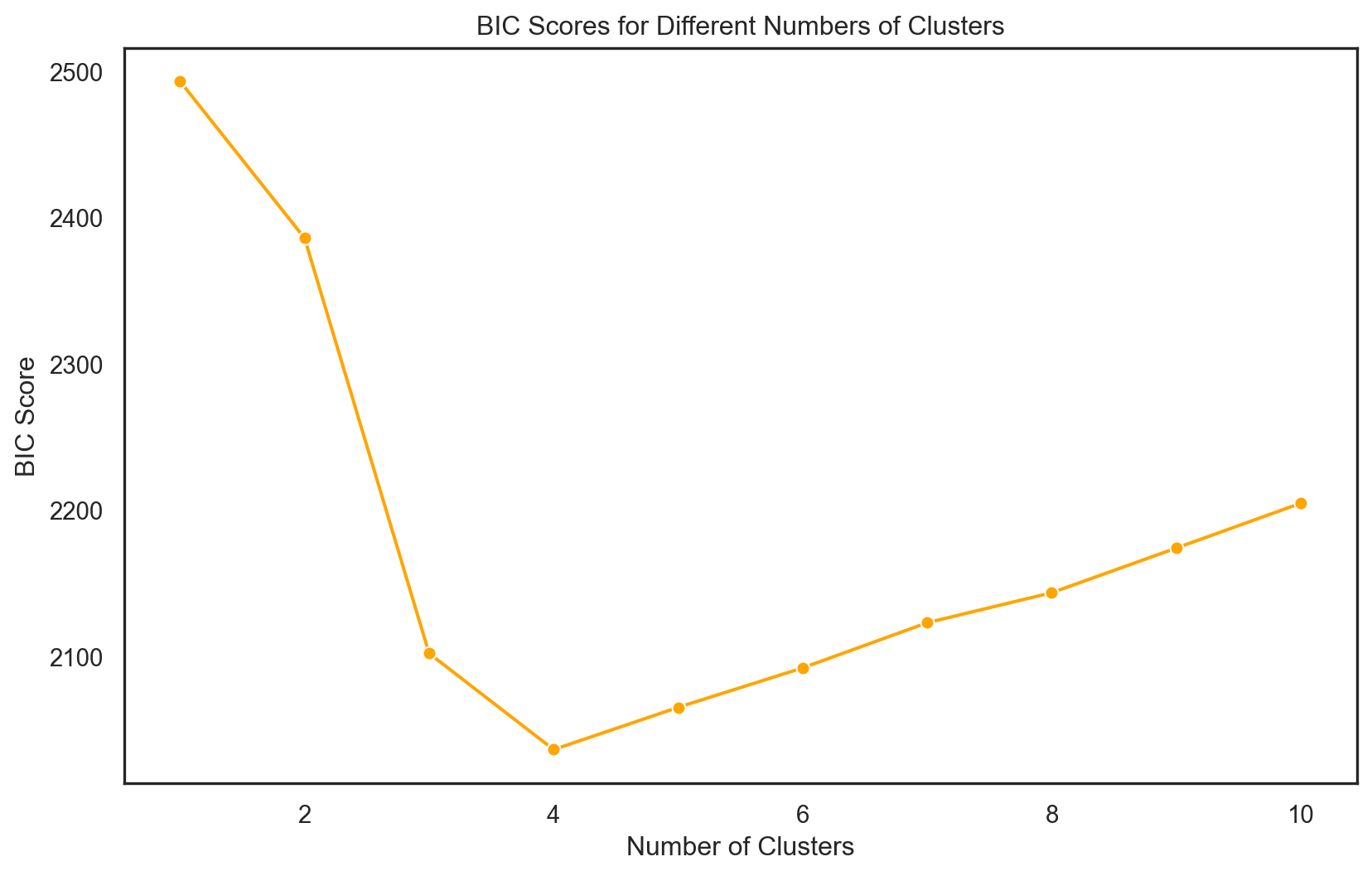
\(\text{BIC} = -2 \ln(\hat{L}) + k \ln(n)\)
where:
\(\hat{L}\) is the maximized value of the likelihood function of the model,
\(k\) is the number of parameters in the model,
\(n\) is the number of observations.
Pros:
Penalizes Complexity: Helps avoid overfitting by penalizing models with more parameters.
Objective Selection: Facilitates choosing the model with the best balance between fit and simplicity.
Applicability: Useful across various model types, including clustering and regression.
Cons:
Computationally Intensive: Requires fitting multiple models to calculate, which can be resource-heavy.
Sensitivity to Model Assumptions: Performance depends on the underlying assumptions of the model being correct.
Not Always Intuitive: Determining the absolute best model may still require domain knowledge and additional diagnostics.
K-Means Clustering: applied
Code
# Finding the optimal number of clusters using Calinski-Harabasz Index
calinski_harabasz_scores = []
cluster_range = range(2, 11)  # Define the range for number of clusters

for n_clusters in cluster_range:
    kmeans = KMeans(n_clusters=n_clusters, random_state=0)
    kmeans.fit(data)
    labels = kmeans.labels_
    score = calinski_harabasz_score(data, labels)
    calinski_harabasz_scores.append(score)

# Plotting the Calinski-Harabasz scores
plt.plot(cluster_range, calinski_harabasz_scores, marker='o')
plt.title('Calinski-Harabasz Index for Different Numbers of Clusters')
plt.xlabel('Number of Clusters')
plt.ylabel('Calinski-Harabasz Index')
plt.grid(True)
plt.show()

# Finding the number of clusters that maximizes the Calinski-Harabasz Index
optimal_n_clusters = cluster_range[calinski_harabasz_scores.index(max(calinski_harabasz_scores))]
print(f"The optimal number of clusters is: {optimal_n_clusters}")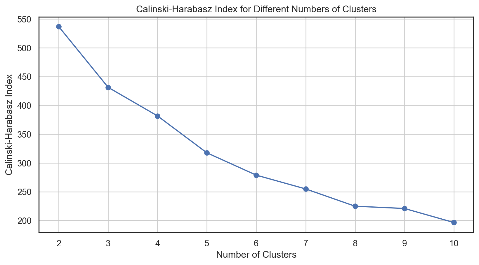
The optimal number of clusters is: 2Code
# K-Means Clustering with the optimal number of clusters
kmeans = KMeans(n_clusters=optimal_n_clusters, random_state=0)
kmeans.fit(data)
clusters = kmeans.predict(data)

# Adding cluster labels to the DataFrame
data['Cluster'] = clusters

# Model Summary
print("Cluster Centers:\n", kmeans.cluster_centers_)

# Evaluate clustering performance using the Calinski-Harabasz Index
calinski_harabasz_score_final = calinski_harabasz_score(data.drop(columns='Cluster'), clusters)
print(f"For n_clusters = {optimal_n_clusters}, the Calinski-Harabasz Index is : {calinski_harabasz_score_final:.3f}")
Cluster Centers:
[[ 6.81306346 0.19993757 -0.28806769 -0.29502272 -0.46716703 0.05454598
-0.12994433 0.03657521 -0.02176455 0.03151719 0.24393655 -0.01449253
-0.03272898 0.04760448 -0.01648803 -0.03251455 0.01440017 0.05300893
-0.01630804]
[-3.57757098 -0.10498814 0.15126567 0.15491779 0.24531156 -0.02864235
0.06823436 -0.01920581 0.01142867 -0.01654982 -0.12809221 0.0076101
0.01718614 -0.02499733 0.00865794 0.01707354 -0.00756159 -0.02783523
0.00856343]]
For n_clusters = 2, the Calinski-Harabasz Index is : 536.957Code
pca = PCA(n_components = 2)
reduced_data_PCA = pca.fit_transform(data)
sns.scatterplot(x = reduced_data_PCA[:, 0], y = reduced_data_PCA[:, 1], hue = clusters, alpha = 0.75, palette = "colorblind")
plt.title('Human Freedom Index Clustered (PCA-reduced Features)')
plt.xlabel('PCA 1')
plt.ylabel('PCA 2')
plt.legend(title = 'Cluster')
plt.show()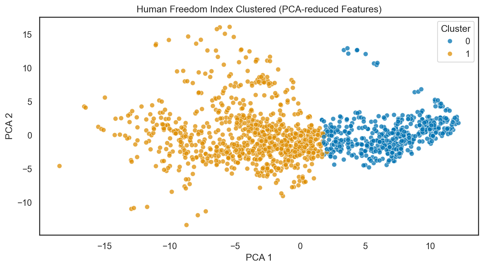
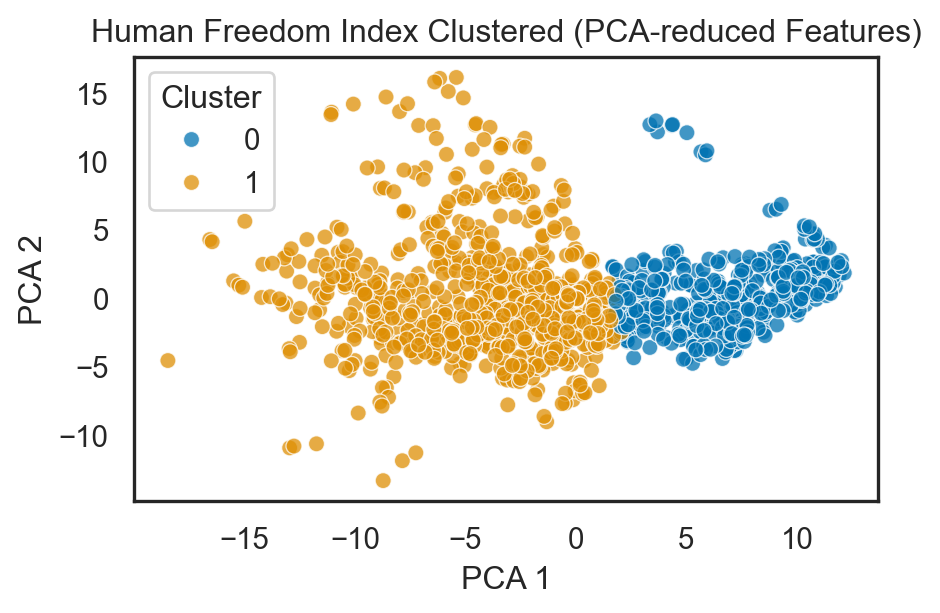
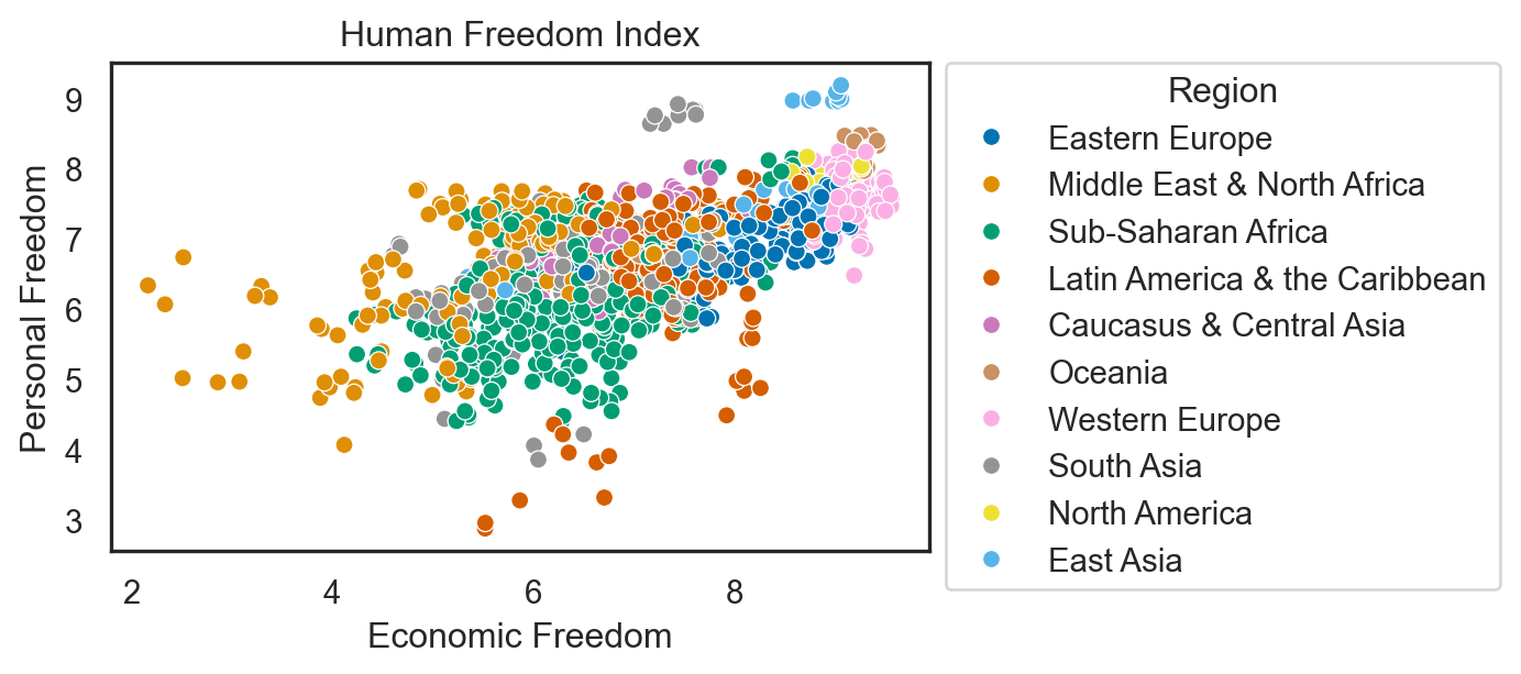
Caveat
Conclusions
Clear Separation:
- Two distinct clusters (Cluster 0 and Cluster 1) are evident, indicating effective separation by PCA.
Cluster Characteristics:
Cluster 1 (orange) is compact and concentrated around the origin.
Cluster 0 (blue) is more spread out across the PCA axes.
Slight Overlap:
- There is a transition zone between the clusters, suggesting some borderline cases.
PCA Components:
- The axes represent the first two principal components, highlighting significant differences in the clusters.
Implications:
- The clusters likely reflect differences in Human Freedom Index scores, with further analysis needed to understand specific feature contributions.
